Graphique pca biplot avec ggplot2
je me demande s'il est possible de tracer les résultats du biplot pca avec ggplot2. Supposons que je veuille afficher les résultats de biplot suivants avec ggplot2
fit <- princomp(USArrests, cor=TRUE)
summary(fit)
biplot(fit)
Toute aide sera très appréciée. Merci
5 réponses
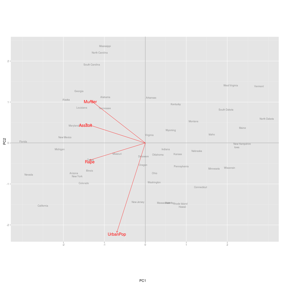
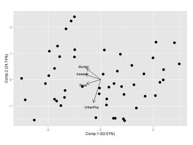
peut-être que cela aidera-- c'est adapté du code que j'ai écrit il y a quelque temps. Il dessine maintenant des flèches ainsi.
PCbiplot <- function(PC, x="PC1", y="PC2") {
    # PC being a prcomp object
    data <- data.frame(obsnames=row.names(PC$x), PC$x)
    plot <- ggplot(data, aes_string(x=x, y=y)) + geom_text(alpha=.4, size=3, aes(label=obsnames))
    plot <- plot + geom_hline(aes(0), size=.2) + geom_vline(aes(0), size=.2)
    datapc <- data.frame(varnames=rownames(PC$rotation), PC$rotation)
    mult <- min(
        (max(data[,y]) - min(data[,y])/(max(datapc[,y])-min(datapc[,y]))),
        (max(data[,x]) - min(data[,x])/(max(datapc[,x])-min(datapc[,x])))
        )
    datapc <- transform(datapc,
            v1 = .7 * mult * (get(x)),
            v2 = .7 * mult * (get(y))
            )
    plot <- plot + coord_equal() + geom_text(data=datapc, aes(x=v1, y=v2, label=varnames), size = 5, vjust=1, color="red")
    plot <- plot + geom_segment(data=datapc, aes(x=0, y=0, xend=v1, yend=v2), arrow=arrow(length=unit(0.2,"cm")), alpha=0.75, color="red")
    plot
}

fit <- prcomp(USArrests, scale=T)
PCbiplot(fit)
Vous pouvez modifier la taille du texte, ainsi que la transparence et les couleurs, le goût; il serait facile de rendre les paramètres de la fonction.
Remarque: il m'est apparu que cela fonctionne avec prcomp mais votre exemple est avec princomp. Vous devrez peut-être, encore une fois, adapter le code en conséquence.
Note 2: code pour geom_segment() est emprunté à la liste de diffusion liée au commentaire to OP.
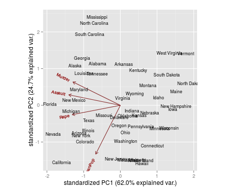
voici le chemin le plus simple à travers ggbiplot:
library(ggbiplot)
fit <- princomp(USArrests, cor=TRUE)
biplot(fit)
ggbiplot(fit, labels = rownames(USArrests))
Si vous utilisez l'excellent FactoMineR paquet pour pca, vous pourriez trouver cela utile pour faire des tracés avec ggplot2
# Plotting the output of FactoMineR's PCA using ggplot2
#
# load libraries
library(FactoMineR)
library(ggplot2)
library(scales)
library(grid)
library(plyr)
library(gridExtra)
#
# start with a clean slate
rm(list=ls(all=TRUE))
#
# load example data from the FactoMineR package
data(decathlon)
#
# compute PCA
res.pca <- PCA(decathlon, quanti.sup = 11:12, quali.sup=13, graph = FALSE)
#
# extract some parts for plotting
PC1 <- res.pca$ind$coord[,1]
PC2 <- res.pca$ind$coord[,2]
labs <- rownames(res.pca$ind$coord)
PCs <- data.frame(cbind(PC1,PC2))
rownames(PCs) <- labs
#
# Just showing the individual samples...
ggplot(PCs, aes(PC1,PC2, label=rownames(PCs))) +
geom_text()
#
# Now get supplementary categorical variables
cPC1 <- res.pca$quali.sup$coor[,1]
cPC2 <- res.pca$quali.sup$coor[,2]
clabs <- rownames(res.pca$quali.sup$coor)
cPCs <- data.frame(cbind(cPC1,cPC2))
rownames(cPCs) <- clabs
colnames(cPCs) <- colnames(PCs)
#
# Put samples and categorical variables (ie. grouping
# of samples) all together
p <- ggplot() + opts(aspect.ratio=1) + theme_bw(base_size = 20)
# no data so there's nothing to plot...
# add on data
p <- p + geom_text(data=PCs, aes(x=PC1,y=PC2,label=rownames(PCs)), size=4)
p <- p + geom_text(data=cPCs, aes(x=cPC1,y=cPC2,label=rownames(cPCs)),size=10)
p # show plot with both layers
#
# clear the plot
dev.off()
#
# Now extract variables
#
vPC1 <- res.pca$var$coord[,1]
vPC2 <- res.pca$var$coord[,2]
vlabs <- rownames(res.pca$var$coord)
vPCs <- data.frame(cbind(vPC1,vPC2))
rownames(vPCs) <- vlabs
colnames(vPCs) <- colnames(PCs)
#
# and plot them
#
pv <- ggplot() + opts(aspect.ratio=1) + theme_bw(base_size = 20)
# no data so there's nothing to plot
# put a faint circle there, as is customary
angle <- seq(-pi, pi, length = 50)
df <- data.frame(x = sin(angle), y = cos(angle))
pv <- pv + geom_path(aes(x, y), data = df, colour="grey70")
#
# add on arrows and variable labels
pv <- pv + geom_text(data=vPCs, aes(x=vPC1,y=vPC2,label=rownames(vPCs)), size=4) + xlab("PC1") + ylab("PC2")
pv <- pv + geom_segment(data=vPCs, aes(x = 0, y = 0, xend = vPC1*0.9, yend = vPC2*0.9), arrow = arrow(length = unit(1/2, 'picas')), color = "grey30")
pv # show plot
#
# clear the plot
dev.off()
#
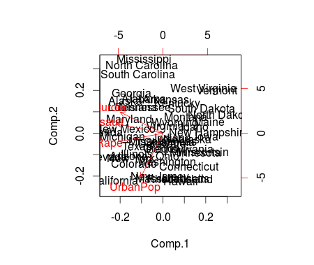
# Now put them side by side
#
library(gridExtra)
grid.arrange(p,pv,nrow=1)
#
# Now they can be saved or exported...
#
# tidy up by deleting the plots
#
dev.off()
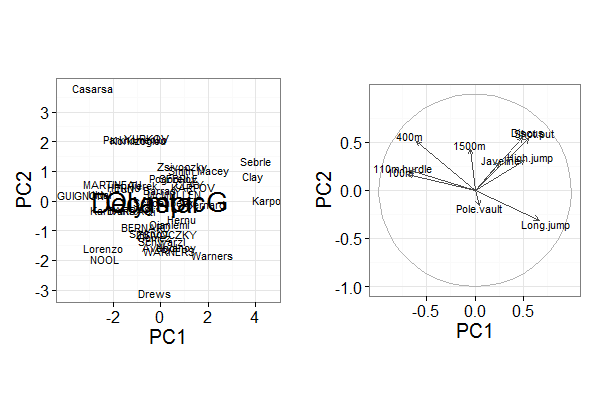
et voici à quoi ressemblent les tracés finaux, peut-être que la taille du texte sur le tracé de gauche pourrait être un peu plus petite:
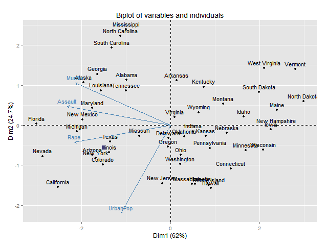
vous pouvez aussi utiliser factoextra qui a aussi un ggplot2 backend:
library("devtools")
install_github("kassambara/factoextra")
fit <- princomp(USArrests, cor=TRUE)
fviz_pca_biplot(fit)
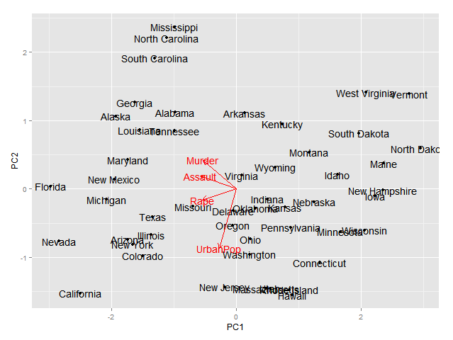
Ou ggord:
install_github('fawda123/ggord')
library(ggord)
ggord(fit)+theme_grey()
Ou ggfortify:
devtools::install_github("sinhrks/ggfortify")
library(ggfortify)
ggplot2::autoplot(fit, label = TRUE, loadings.label = TRUE)
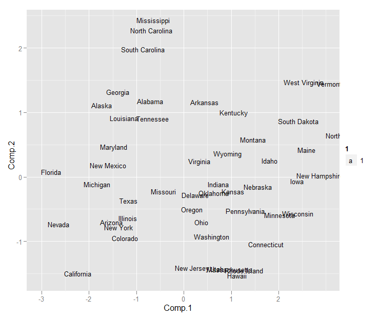
cela permet de tracer les États, mais pas les variables
fit.df <- as.data.frame(fit$scores)
fit.df$state <- rownames(fit.df)

library(ggplot2)
ggplot(data=fit.df,aes(x=Comp.1,y=Comp.2))+
  geom_text(aes(label=state,size=1,hjust=0,vjust=0))