Joindre un dendrogramme et une heatmap

Question

Joindre un dendrogramme et une heatmap

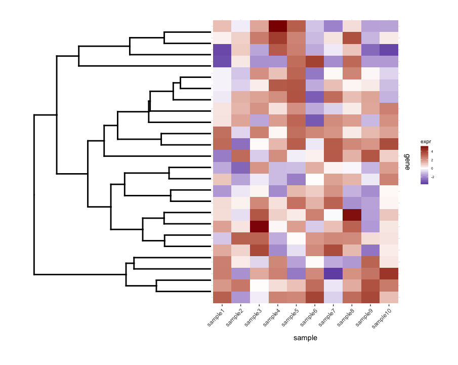
j'ai un heatmap (expression de gènes à partir d'un ensemble d'échantillons):

set.seed(10)
mat <- matrix(rnorm(24*10,mean=1,sd=2),nrow=24,ncol=10,dimnames=list(paste("g",1:24,sep=""),paste("sample",1:10,sep="")))
dend <- as.dendrogram(hclust(dist(mat)))
row.ord <- order.dendrogram(dend)
mat <- matrix(mat[row.ord,],nrow=24,ncol=10,dimnames=list(rownames(mat)[row.ord],colnames(mat)))
mat.df <- reshape2::melt(mat,value.name="expr",varnames=c("gene","sample"))

require(ggplot2)
map1.plot <- ggplot(mat.df,aes(x=sample,y=gene))+geom_tile(aes(fill=expr))+scale_fill_gradient2("expr",high="darkred",low="darkblue")+scale_y_discrete(position="right")+
  theme_bw()+theme(plot.margin=unit(c(1,1,1,-1),"cm"),legend.key=element_blank(),legend.position="right",axis.text.y=element_blank(),axis.ticks.y=element_blank(),panel.border=element_blank(),strip.background=element_blank(),axis.text.x=element_text(angle=45,hjust=1,vjust=1),legend.text=element_text(size=5),legend.title=element_text(size=8),legend.key.size=unit(0.4,"cm"))

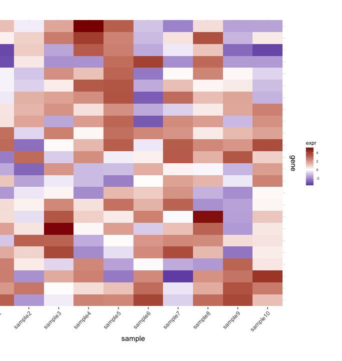
(le côté gauche est coupé à cause du plot.margin arguments que j'utilise mais j'en ai besoin pour ce qui est montré ci-dessous).

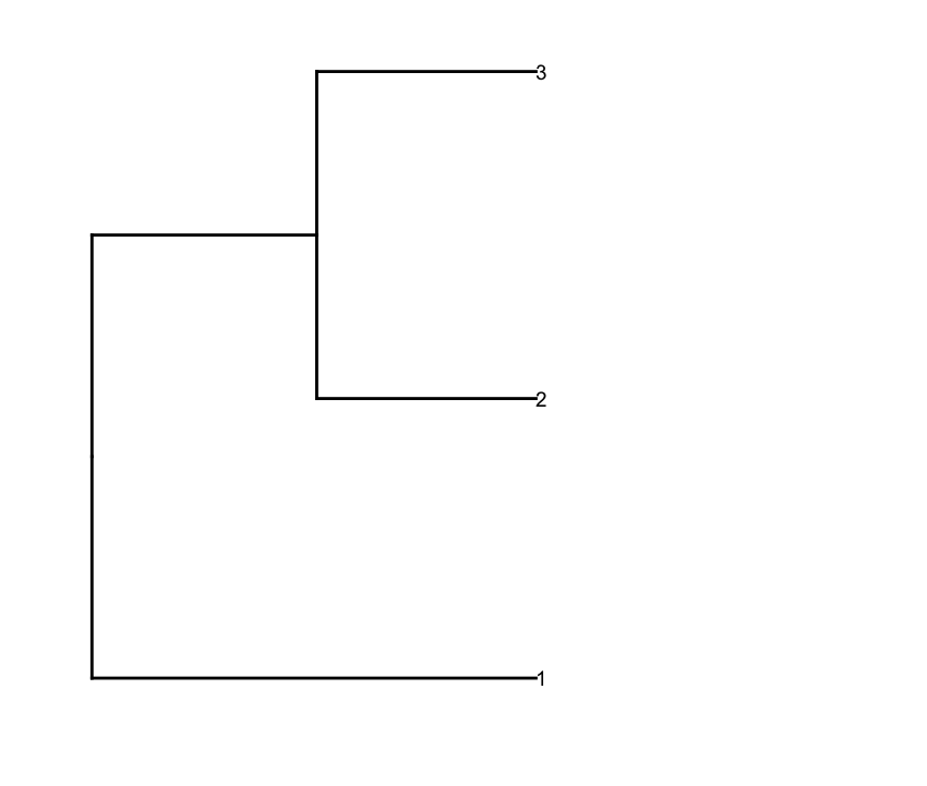
Puis-Je prune la ligne dendrogram selon une valeur de coupure de profondeur pour obtenir moins de clusters (i.e., seulement Deep splits), et faire un peu d'édition sur le résultat dendrogram pour avoir comploté la façon que je veux c':

depth.cutoff <- 11
dend <- cut(dend,h=depth.cutoff)$upper
require(dendextend)
gg.dend <- as.ggdend(dend)
leaf.heights <- dplyr::filter(gg.dend$nodes,!is.na(leaf))$height
leaf.seqments.idx <- which(gg.dend$segments$yend %in% leaf.heights)
gg.dend$segments$yend[leaf.seqments.idx] <- max(gg.dend$segments$yend[leaf.seqments.idx])
gg.dend$segments$col[leaf.seqments.idx] <- "black"
gg.dend$labels$label <- 1:nrow(gg.dend$labels)
gg.dend$labels$y <- max(gg.dend$segments$yend[leaf.seqments.idx])
gg.dend$labels$x <- gg.dend$segments$x[leaf.seqments.idx]
gg.dend$labels$col <- "black"
dend1.plot <- ggplot(gg.dend,labels=F)+scale_y_reverse()+coord_flip()+theme(plot.margin=unit(c(1,-3,1,1),"cm"))+annotate("text",size=5,hjust=0,x=gg.dend$label$x,y=gg.dend$label$y,label=gg.dend$label$label,colour=gg.dend$label$col)

Et j'ai tracé à l'aide d' cowplotplot_grid:

require(cowplot)
plot_grid(dend1.plot,map1.plot,align='h',rel_widths=c(0.5,1))

Bien que le align='h' travaille, il n'est pas parfait.

traçant le non-découpé dendrogrammap1.plot en utilisant plot_grid illustre cela:

dend0.plot <- ggplot(as.ggdend(dend))+scale_y_reverse()+coord_flip()+theme(plot.margin=unit(c(1,-1,1,1),"cm"))
plot_grid(dend0.plot,map1.plot,align='h',rel_widths=c(1,1))

Les branches en haut et en bas de l' dendrogram semblent être écrasé vers le centre. En jouant avec les scale semble être une façon de l'ajuster, mais les valeurs de l'échelle semblent être spécifiques à la figure, donc je me demande s'il y a un moyen de le faire d'une manière plus basée sur des principes.

Ensuite, je fais quelques terme d'enrichissement de l'analyse sur chaque cluster de mon heatmap. Supposons que cette analyse m'ait donné ceci!--23-->:

enrichment.df <- data.frame(term=rep(paste("t",1:10,sep=""),nrow(gg.dend$labels)),
                          cluster=c(sapply(1:nrow(gg.dend$labels),function(i) rep(i,5))),
                          score=rgamma(10*nrow(gg.dend$labels),0.2,0.7),
                          stringsAsFactors = F)

Ce que je voudrais faire est de tracer ce data.frameheatmap et le lieu de la couper dendrogram - dessous (de la même manière qu'il est placé à gauche de l'expression heatmap).

alors j'ai essayé plot_grid nouveau penser que align='v' travail ici:

d'abord régénérer la parcelle de dendrogramme en lui faisant face vers le haut:

dend2.plot <- ggplot(gg.dend,labels=F)+scale_y_reverse()+theme(plot.margin=unit(c(-3,1,1,1),"cm"))

maintenant, j'essaie de les rassembler:

plot_grid(map2.plot,dend2.plot,align='v')

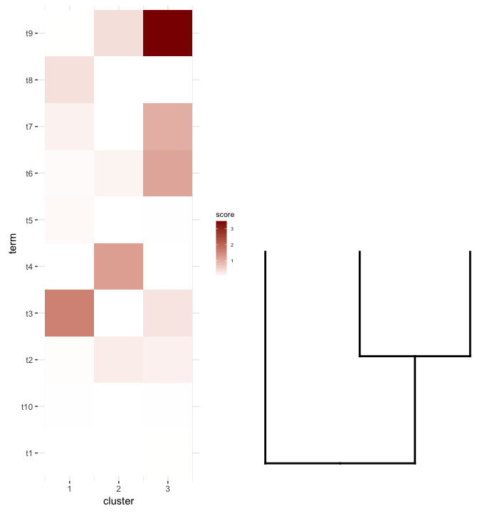
plot_grid ne semble pas capable de les aligner comme le montre la figure et le message d'avertissement lancers:

In align_plots(plotlist = plots, align = align) :
  Graphs cannot be vertically aligned. Placing graphs unaligned.

Ce qui ne semble pas obtenir près, c'est ceci:

plot_grid(map2.plot,dend2.plot,rel_heights=c(1,0.5),nrow=2,ncol=1,scale=c(1,0.675))

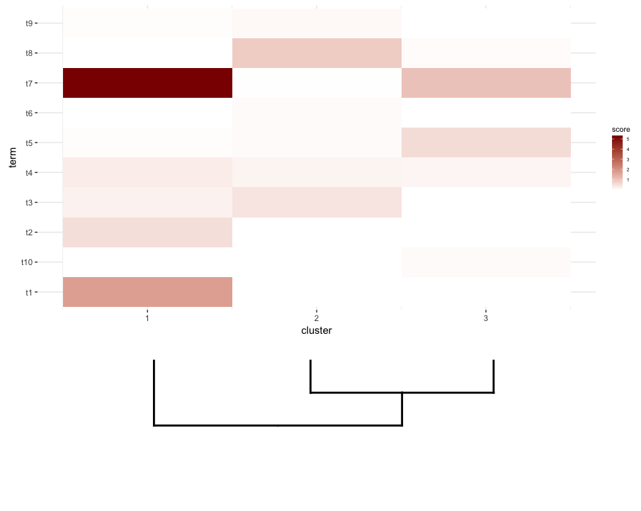
Ceci est réalisé après avoir joué avec les scale paramètre, bien que l'intrigue sort trop large. Encore une fois, je me demande s'il y a un moyen de contourner ou de prédéfinir ce qui est correct scale pour une liste de dendrogram et heatmap, peut-être par leurs dimensions.

23

cowplot dendrogram ggplot2 heatmap r

demandé sur Axeman 2017-02-05 05:17:14

2 réponses

score 10 · Answer 1

j'ai eu à peu près le même problème il y a quelque temps. L'astuce de base que j'ai utilisé était de spécifier directement les positions des gènes, étant donné les résultats du dendrogramme. Par souci de simplicité, voici d'abord le cas du tracé du dendrogramme complet:

# For the full dendrogram
library(plyr)
library(reshape2)
library(dplyr)
library(ggplot2)
library(ggdendro)
library(gridExtra)
library(dendextend)

set.seed(10)

# The source data
mat <- matrix(rnorm(24 * 10, mean = 1, sd = 2), 
              nrow = 24, ncol = 10, 
              dimnames = list(paste("g", 1:24, sep = ""), 
                              paste("sample", 1:10, sep = "")))

sample_names <- colnames(mat)

# Obtain the dendrogram
dend <- as.dendrogram(hclust(dist(mat)))
dend_data <- dendro_data(dend)

# Setup the data, so that the layout is inverted (this is more 
# "clear" than simply using coord_flip())
segment_data <- with(
    segment(dend_data), 
    data.frame(x = y, y = x, xend = yend, yend = xend))
# Use the dendrogram label data to position the gene labels
gene_pos_table <- with(
    dend_data$labels, 
    data.frame(y_center = x, gene = as.character(label), height = 1))

# Table to position the samples
sample_pos_table <- data.frame(sample = sample_names) %>%
    mutate(x_center = (1:n()), 
           width = 1)

# Neglecting the gap parameters
heatmap_data <- mat %>% 
    reshape2::melt(value.name = "expr", varnames = c("gene", "sample")) %>%
    left_join(gene_pos_table) %>%
    left_join(sample_pos_table)

# Limits for the vertical axes
gene_axis_limits <- with(
    gene_pos_table, 
    c(min(y_center - 0.5 * height), max(y_center + 0.5 * height))
) + 
    0.1 * c(-1, 1) # extra spacing: 0.1

# Heatmap plot
plt_hmap <- ggplot(heatmap_data, 
                   aes(x = x_center, y = y_center, fill = expr, 
                       height = height, width = width)) + 
    geom_tile() +
    scale_fill_gradient2("expr", high = "darkred", low = "darkblue") +
    scale_x_continuous(breaks = sample_pos_table$x_center, 
                       labels = sample_pos_table$sample, 
                       expand = c(0, 0)) + 
    # For the y axis, alternatively set the labels as: gene_position_table$gene
    scale_y_continuous(breaks = gene_pos_table[, "y_center"], 
                       labels = rep("", nrow(gene_pos_table)),
                       limits = gene_axis_limits, 
                       expand = c(0, 0)) + 
    labs(x = "Sample", y = "") +
    theme_bw() +
    theme(axis.text.x = element_text(size = rel(1), hjust = 1, angle = 45), 
          # margin: top, right, bottom, and left
          plot.margin = unit(c(1, 0.2, 0.2, -0.7), "cm"), 
          panel.grid.minor = element_blank())

# Dendrogram plot
plt_dendr <- ggplot(segment_data) + 
    geom_segment(aes(x = x, y = y, xend = xend, yend = yend)) + 
    scale_x_reverse(expand = c(0, 0.5)) + 
    scale_y_continuous(breaks = gene_pos_table$y_center, 
                       labels = gene_pos_table$gene, 
                       limits = gene_axis_limits, 
                       expand = c(0, 0)) + 
    labs(x = "Distance", y = "", colour = "", size = "") +
    theme_bw() + 
    theme(panel.grid.minor = element_blank())

library(cowplot)
plot_grid(plt_dendr, plt_hmap, align = 'h', rel_widths = c(1, 1))

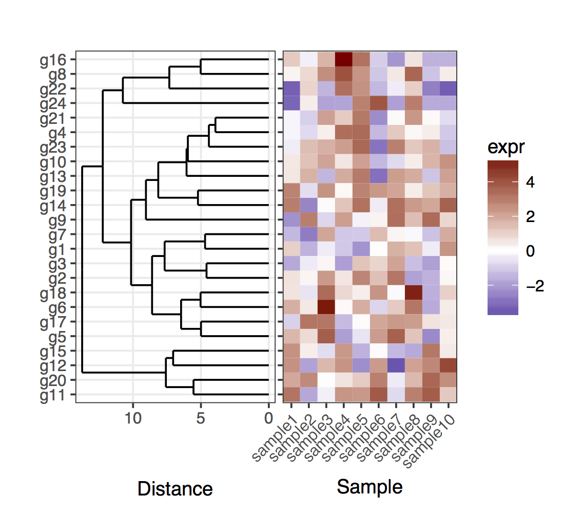
notez que j'ai gardé les tiques de l'axe des y à gauche dans le tracé heatmap, juste pour montrer que le dendrogramme et les tiques correspondent exactement.

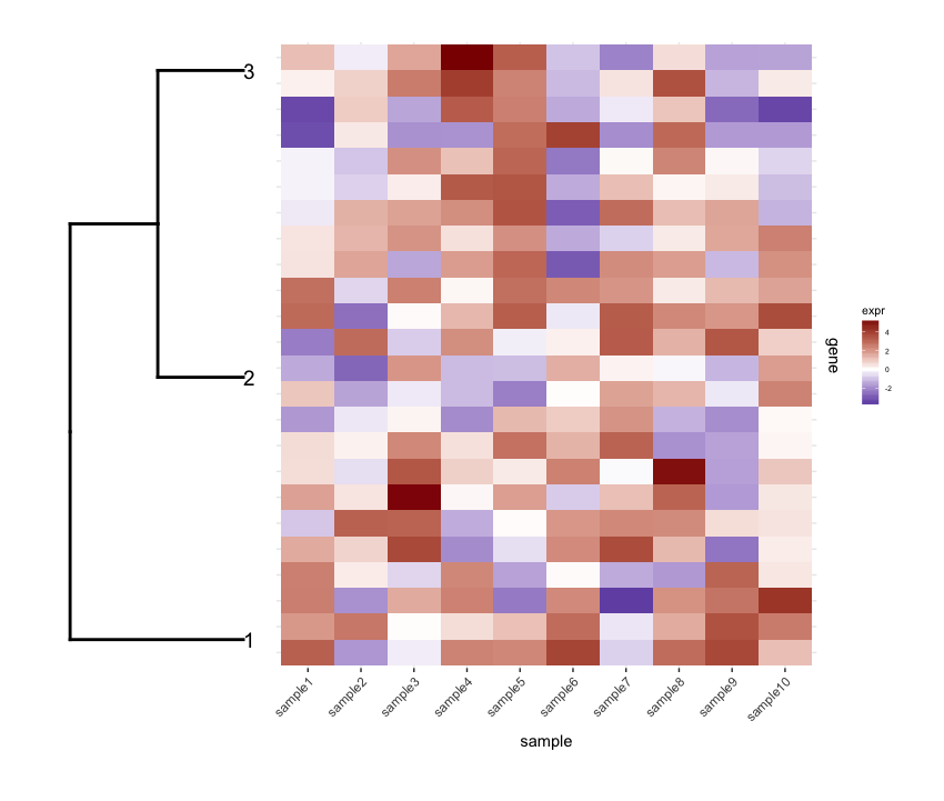
Maintenant, pour le cas de le dendrogramme coupé, il faut garder à l'esprit que les feuilles du dendrogramme ne se termineront plus dans la position exacte correspondant à un gène dans un cluster donné. Pour obtenir les positions des gènes et des amas, il faut extraire les données des deux dendrogrammes qui résultent de la coupe complète. Dans l'ensemble, pour clarifier les gènes dans les amas, j'ai ajouté des rectangles qui délimitent les amas.

# For the cut dendrogram
library(plyr)
library(reshape2)
library(dplyr)
library(ggplot2)
library(ggdendro)
library(gridExtra)
library(dendextend)

set.seed(10)

# The source data
mat <- matrix(rnorm(24 * 10, mean = 1, sd = 2), 
              nrow = 24, ncol = 10, 
              dimnames = list(paste("g", 1:24, sep = ""), 
                              paste("sample", 1:10, sep = "")))

sample_names <- colnames(mat)

# Obtain the dendrogram
full_dend <- as.dendrogram(hclust(dist(mat)))

# Cut the dendrogram
depth_cutoff <- 11
h_c_cut <- cut(full_dend, h = depth_cutoff)
dend_cut <- as.dendrogram(h_c_cut$upper)
dend_cut <- hang.dendrogram(dend_cut)
# Format to extend the branches (optional)
dend_cut <- hang.dendrogram(dend_cut, hang = -1) 
dend_data_cut <- dendro_data(dend_cut)

# Extract the names assigned to the clusters (e.g., "Branch 1", "Branch 2", ...)
cluster_names <- as.character(dend_data_cut$labels$label)
# Extract the names of the haplotypes that belong to each group (using
# the 'labels' function)
lst_genes_in_clusters <- h_c_cut$lower %>% 
    lapply(labels) %>% 
    setNames(cluster_names)

# Setup the data, so that the layout is inverted (this is more 
# "clear" than simply using coord_flip())
segment_data <- with(
    segment(dend_data_cut), 
    data.frame(x = y, y = x, xend = yend, yend = xend))

# Extract the positions of the clusters (by getting the positions of the 
# leafs); data is already in the same order as in the cluster name
cluster_positions <- segment_data[segment_data$xend == 0, "y"]
cluster_pos_table <- data.frame(y_position = cluster_positions, 
                                cluster = cluster_names)

# Specify the positions for the genes, accounting for the clusters
gene_pos_table <- lst_genes_in_clusters %>%
    ldply(function(ss) data.frame(gene = ss), .id = "cluster") %>%
    mutate(y_center = 1:nrow(.), 
           height = 1)
# > head(gene_pos_table, 3)
#    cluster gene y_center height
# 1 Branch 1  g11        1      1
# 2 Branch 1  g20        2      1
# 3 Branch 1  g12        3      1

# Table to position the samples
sample_pos_table <- data.frame(sample = sample_names) %>%
    mutate(x_center = 1:nrow(.), 
           width = 1)

# Coordinates for plotting rectangles delimiting the clusters: aggregate
# over the positions of the genes in each cluster
cluster_delim_table <- gene_pos_table %>%
    group_by(cluster) %>%
    summarize(y_min = min(y_center - 0.5 * height), 
              y_max = max(y_center + 0.5 * height)) %>%
    as.data.frame() %>%
    mutate(x_min = with(sample_pos_table, min(x_center - 0.5 * width)), 
           x_max = with(sample_pos_table, max(x_center + 0.5 * width)))

# Neglecting the gap parameters
heatmap_data <- mat %>% 
    reshape2::melt(value.name = "expr", varnames = c("gene", "sample")) %>%
    left_join(gene_pos_table) %>%
    left_join(sample_pos_table)

# Limits for the vertical axes (genes / clusters)
gene_axis_limits <- with(
    gene_pos_table, 
    c(min(y_center - 0.5 * height), max(y_center + 0.5 * height))
) + 
    0.1 * c(-1, 1) # extra spacing: 0.1

# Heatmap plot
plt_hmap <- ggplot(heatmap_data, 
                   aes(x = x_center, y = y_center, fill = expr, 
                       height = height, width = width)) + 
    geom_tile() +
    geom_rect(data = cluster_delim_table, 
              aes(xmin = x_min, xmax = x_max, ymin = y_min, ymax = y_max), 
              fill = NA, colour = "black", inherit.aes = FALSE) + 
    scale_fill_gradient2("expr", high = "darkred", low = "darkblue") +
    scale_x_continuous(breaks = sample_pos_table$x_center, 
                       labels = sample_pos_table$sample, 
                       expand = c(0.01, 0.01)) + 
    scale_y_continuous(breaks = gene_pos_table$y_center, 
                       labels = gene_pos_table$gene, 
                       limits = gene_axis_limits, 
                       expand = c(0, 0), 
                       position = "right") + 
    labs(x = "Sample", y = "") +
    theme_bw() +
    theme(axis.text.x = element_text(size = rel(1), hjust = 1, angle = 45), 
          # margin: top, right, bottom, and left
          plot.margin = unit(c(1, 0.2, 0.2, -0.1), "cm"), 
          panel.grid.minor = element_blank())

# Dendrogram plot
plt_dendr <- ggplot(segment_data) + 
    geom_segment(aes(x = x, y = y, xend = xend, yend = yend)) + 
    scale_x_reverse(expand = c(0, 0.5)) + 
    scale_y_continuous(breaks = cluster_pos_table$y_position, 
                       labels = cluster_pos_table$cluster, 
                       limits = gene_axis_limits, 
                       expand = c(0, 0)) + 
    labs(x = "Distance", y = "", colour = "", size = "") +
    theme_bw() + 
    theme(panel.grid.minor = element_blank())

library(cowplot)
plot_grid(plt_dendr, plt_hmap, align = 'h', rel_widths = c(1, 1.8))

score 1 · Answer 2

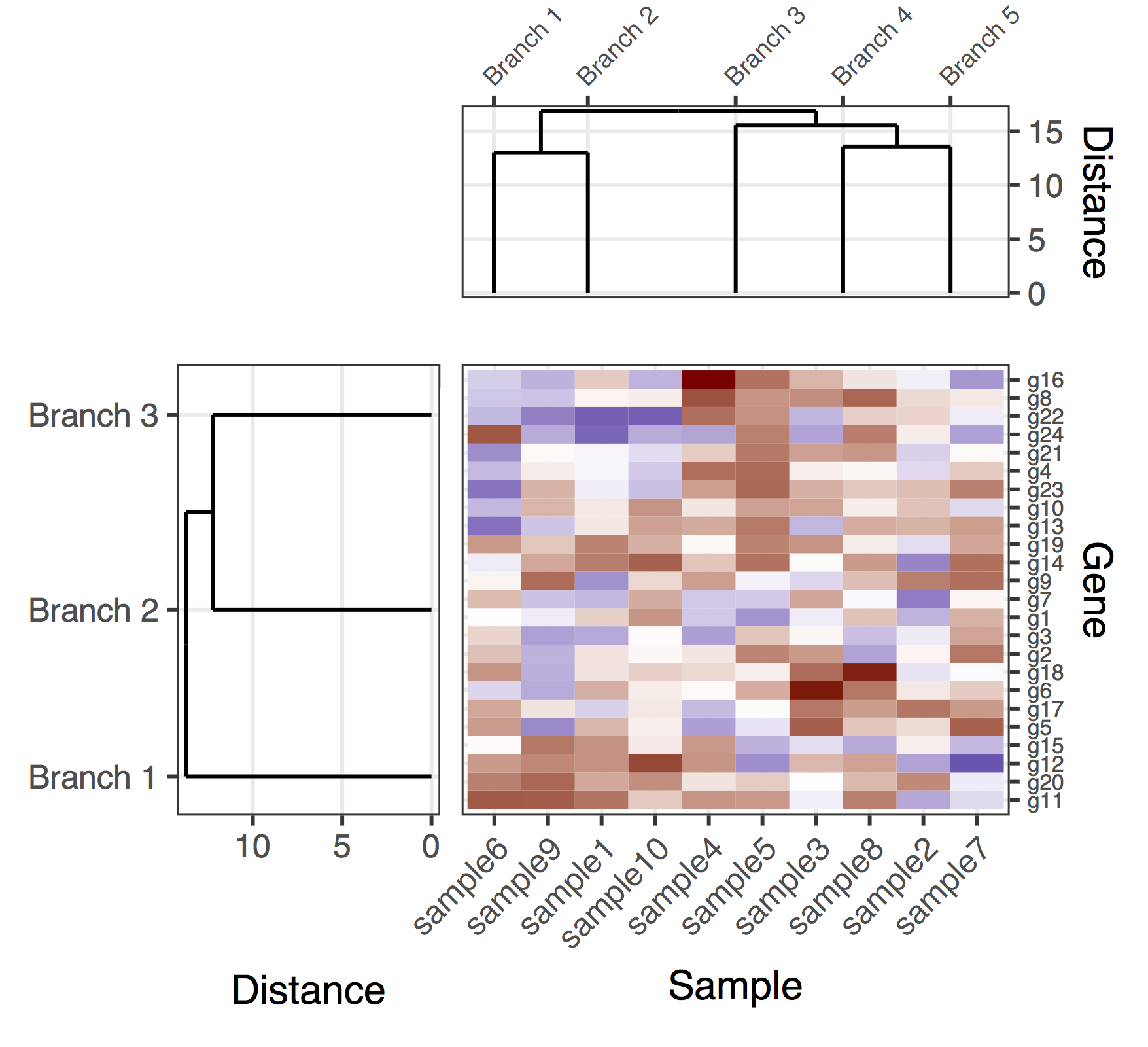
Voici une solution (provisoire) avec le gène et les dendrogrammes d'échantillon. C'est une solution plutôt manquante, parce que je n'ai pas réussi à trouver un bon moyen d'obtenir plot_grid pour aligner correctement tous les sous-lots, tout en ajustant automatiquement les proportions des figures et les distances entre les sous-parcelles. Dans cette version, la façon de produire la figure globale était d'ajouter "padding subplots" (les entrées nulles flanquant dans l'appel à plot_grid) et également régler manuellement les marges des sous-parcelles (qui étrangement semble être couplé dans les différents sous-lots). Une fois de plus, il s'agit d'une solution plutôt manquant, j'espère que je peux arriver à poster une version définitive bientôt.

library(plyr)
library(reshape2)
library(dplyr)
library(ggplot2)
library(ggdendro)
library(gridExtra)
library(dendextend)

set.seed(10)

# The source data
mat <- matrix(rnorm(24 * 10, mean = 1, sd = 2), 
              nrow = 24, ncol = 10, 
              dimnames = list(paste("g", 1:24, sep = ""), 
                              paste("sample", 1:10, sep = "")))

getDendrogram <- function(data_mat, depth_cutoff) {

    # Obtain the dendrogram
    full_dend <- as.dendrogram(hclust(dist(data_mat)))

    # Cut the dendrogram
    h_c_cut <- cut(full_dend, h = depth_cutoff)
    dend_cut <- as.dendrogram(h_c_cut$upper)
    dend_cut <- hang.dendrogram(dend_cut)
    # Format to extend the branches (optional)
    dend_cut <- hang.dendrogram(dend_cut, hang = -1) 
    dend_data_cut <- dendro_data(dend_cut)

    # Extract the names assigned to the clusters (e.g., "Branch 1", "Branch 2", ...)
    cluster_names <- as.character(dend_data_cut$labels$label)
    # Extract the entries that belong to each group (using the 'labels' function)
    lst_entries_in_clusters <- h_c_cut$lower %>% 
        lapply(labels) %>% 
        setNames(cluster_names)

    # The dendrogram data for plotting
    segment_data <- segment(dend_data_cut)

    # Extract the positions of the clusters (by getting the positions of the 
    # leafs); data is already in the same order as in the cluster name
    cluster_positions <- segment_data[segment_data$yend == 0, "x"]
    cluster_pos_table <- data.frame(position = cluster_positions, 
                                    cluster = cluster_names)

    list(
        full_dend = full_dend, 
        dend_data_cut = dend_data_cut, 

        lst_entries_in_clusters = lst_entries_in_clusters, 
        segment_data = segment_data, 
        cluster_pos_table = cluster_pos_table
    )
}

# Cut the dendrograms
gene_depth_cutoff <- 11
sample_depth_cutof <- 12

# Obtain the dendrograms
gene_dend_data <- getDendrogram(mat, gene_depth_cutoff)
sample_dend_data <- getDendrogram(t(mat), sample_depth_cutof)

# Specify the positions for the genes and samples, accounting for the clusters
gene_pos_table <- gene_dend_data$lst_entries_in_clusters %>%
    ldply(function(ss) data.frame(gene = ss), .id = "gene_cluster") %>%
    mutate(y_center = 1:nrow(.), 
           height = 1)
# > head(gene_pos_table, 3)
#    cluster gene y_center height
# 1 Branch 1  g11        1      1
# 2 Branch 1  g20        2      1
# 3 Branch 1  g12        3      1

# Specify the positions for the samples, accounting for the clusters
sample_pos_table <- sample_dend_data$lst_entries_in_clusters %>%
    ldply(function(ss) data.frame(sample = ss), .id = "sample_cluster") %>%
    mutate(x_center = 1:nrow(.), 
           width = 1)

# Neglecting the gap parameters
heatmap_data <- mat %>% 
    reshape2::melt(value.name = "expr", varnames = c("gene", "sample")) %>%
    left_join(gene_pos_table) %>%
    left_join(sample_pos_table)

# Limits for the vertical axes (genes / clusters)
axis_spacing <- 0.1 * c(-1, 1)
gene_axis_limits <- with(
    gene_pos_table, 
    c(min(y_center - 0.5 * height), max(y_center + 0.5 * height))) + axis_spacing

sample_axis_limits <- with(
    sample_pos_table, 
    c(min(x_center - 0.5 * width), max(x_center + 0.5 * width))) + axis_spacing

# For some reason, the margin of the various sub-plots end up being "coupled"; 
# therefore, for now this requires some manual fine-tuning, 
# which is obviously not ideal...
# margin: top, right, bottom, and left
margin_specs_hmap <- 1 * c(-2, -1, -1, -2)
margin_specs_gene_dendr <- 1.7 * c(-1, -2, -1, -1)
margin_specs_sample_dendr <- 1.7 * c(-2, -1, -2, -1)

# Heatmap plot
plt_hmap <- ggplot(heatmap_data, 
                   aes(x = x_center, y = y_center, fill = expr, 
                       height = height, width = width)) + 
    geom_tile() +
    scale_fill_gradient2("expr", high = "darkred", low = "darkblue") +
    scale_x_continuous(breaks = sample_pos_table$x_center, 
                       labels = sample_pos_table$sample, 
                       expand = c(0.01, 0.01)) + 
    scale_y_continuous(breaks = gene_pos_table$y_center, 
                       labels = gene_pos_table$gene, 
                       limits = gene_axis_limits, 
                       expand = c(0.01, 0.01), 
                       position = "right") + 
    labs(x = "Sample", y = "Gene") +
    theme_bw() +
    theme(axis.text.x = element_text(size = rel(1), hjust = 1, angle = 45), 
          axis.text.y = element_text(size = rel(0.7)), 
          legend.position = "none", 
          plot.margin = unit(margin_specs_hmap, "cm"), 
          panel.grid.minor = element_blank())

# Dendrogram plots
plt_gene_dendr <- ggplot(gene_dend_data$segment_data) + 
    geom_segment(aes(x = y, y = x, xend = yend, yend = xend)) + # inverted coordinates
    scale_x_reverse(expand = c(0, 0.5)) + 
    scale_y_continuous(breaks = gene_dend_data$cluster_pos_table$position, 
                       labels = gene_dend_data$cluster_pos_table$cluster, 
                       limits = gene_axis_limits, 
                       expand = c(0, 0)) + 
    labs(x = "Distance", y = "", colour = "", size = "") +
    theme_bw() + 
    theme(plot.margin = unit(margin_specs_gene_dendr, "cm"), 
          panel.grid.minor = element_blank())

plt_sample_dendr <- ggplot(sample_dend_data$segment_data) + 
    geom_segment(aes(x = x, y = y, xend = xend, yend = yend)) + 
    scale_y_continuous(expand = c(0, 0.5), 
                       position = "right") + 
    scale_x_continuous(breaks = sample_dend_data$cluster_pos_table$position, 
                       labels = sample_dend_data$cluster_pos_table$cluster, 
                       limits = sample_axis_limits, 
                       position = "top", 
                       expand = c(0, 0)) + 
    labs(x = "", y = "Distance", colour = "", size = "") +
    theme_bw() + 
    theme(plot.margin = unit(margin_specs_sample_dendr, "cm"), 
          panel.grid.minor = element_blank(), 
          axis.text.x = element_text(size = rel(0.8), angle = 45, hjust = 0))

library(cowplot)

final_plot <- plot_grid(
    NULL,    NULL,           NULL,             NULL, 
    NULL,    NULL,           plt_sample_dendr, NULL, 
    NULL,    plt_gene_dendr, plt_hmap,         NULL, 
    NULL,    NULL,           NULL,             NULL, 
    nrow = 4, ncol = 4, align = "hv", 
    rel_heights = c(0.5, 1, 2, 0.5), 
    rel_widths = c(0.5, 1, 2, 0.5)
)

Las etiquetas más populares

Joindre un dendrogramme et une heatmap

2 réponses