carte du monde sans rivières avec matplotlib / Basemap?
y aurait-il un moyen de tracer les frontières des continents avec Basemap (ou sans Basemap, s'il y a un autre moyen), sans que ces rivières ennuyeuses ne viennent? Surtout cette partie de la rivière Kongo, qui n'atteint même pas l'océan, est troublante.
EDIT: j'ai l'intention de tracer les données sur la carte, comme dans le bibliothèque (et ont encore les frontières des continents dessinées comme des lignes noires sur les données, pour donner la structure pour le worldmap) ainsi alors que la solution par accroché ci-dessous est agréable, magistral même, il n'est pas applicable à cette fin.
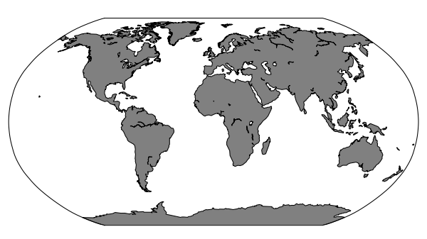
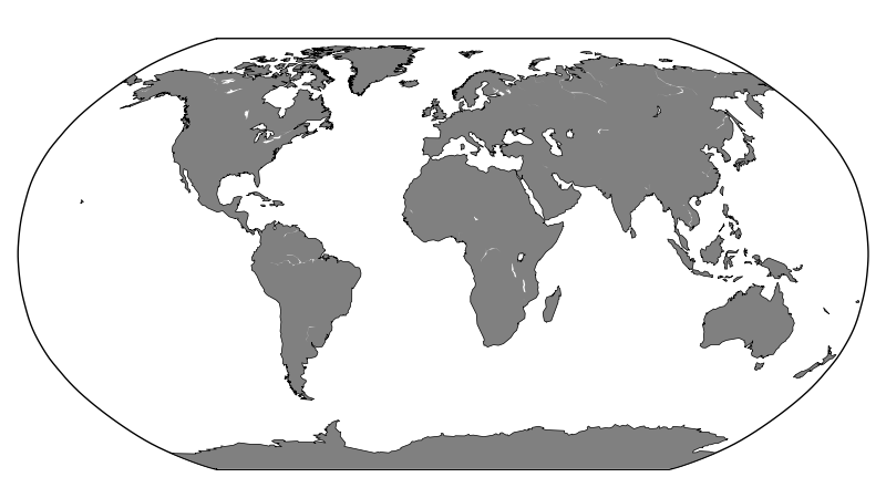
Image produite par:
from mpl_toolkits.basemap import Basemap
import matplotlib.pyplot as plt

fig = plt.figure(figsize=(8, 4.5))
plt.subplots_adjust(left=0.02, right=0.98, top=0.98, bottom=0.00)
m = Basemap(projection='robin',lon_0=0,resolution='c')
m.fillcontinents(color='gray',lake_color='white')
m.drawcoastlines()
plt.savefig('world.png',dpi=75)
7 réponses
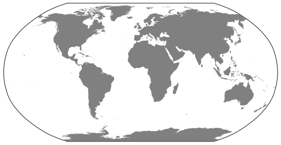
pour des raisons comme celles-ci, j'évite souvent de Basemap alltogether et de lire le shapefile avec OGR et de les convertir en un artiste Matplotlib moi-même. Ce qui est beaucoup plus de travail, mais aussi donne beaucoup plus de flexibilité.
Basemap a quelques traits très soignés comme Convertir les coordonnées des données d'entrée à votre 'projection de travail'.
si vous voulez rester avec Basemap, obtenez un shapefile qui ne contient pas les rivières. La Terre naturelle, par exemple, a un joli shapefile 'Land' la section physique (télécharger les données "scale rank" et décompresser). Voir http://www.naturalearthdata.com/downloads/10m-physical-vectors/
Vous pouvez lire le shapefile avec le M. méthode readshapefile () de Basemap. Cela vous permet d'obtenir les vertices et les codes de chemin Matplotlib dans les coordonnées de projection que vous pouvez ensuite convertir en un nouveau chemin. C'est un peu d'un détour, mais il vous donne toutes les options de style de Matplotlib, dont la plupart ne sont pas directement disponibles via le Fond de carte. C'est un peu hackish, mais je ne maintenant une autre façon tout en restant à Basemap.
Donc:
from mpl_toolkits.basemap import Basemap
import matplotlib.pyplot as plt
from matplotlib.collections import PathCollection
from matplotlib.path import Path

fig = plt.figure(figsize=(8, 4.5))
plt.subplots_adjust(left=0.02, right=0.98, top=0.98, bottom=0.00)

# MPL searches for ne_10m_land.shp in the directory 'D:\ne_10m_land'
m = Basemap(projection='robin',lon_0=0,resolution='c')
shp_info = m.readshapefile('D:\ne_10m_land', 'scalerank', drawbounds=True)
ax = plt.gca()
ax.cla()

paths = []
for line in shp_info[4]._paths:
    paths.append(Path(line.vertices, codes=line.codes))

coll = PathCollection(paths, linewidths=0, facecolors='grey', zorder=2)

m = Basemap(projection='robin',lon_0=0,resolution='c')
# drawing something seems necessary to 'initiate' the map properly
m.drawcoastlines(color='white', zorder=0)

ax = plt.gca()
ax.add_collection(coll)

plt.savefig('world.png',dpi=75)
Donne:
comment supprimer les rivières" agaçantes":
si vous voulez post-traiter l'image (au lieu de travailler directement avec Basemap), vous pouvez enlever les plans d'eau qui ne se connectent pas à l'océan:
import pylab as plt
A = plt.imread("world.png")

import numpy as np
import scipy.ndimage as nd
import collections

# Get a counter of the greyscale colors
a      = A[:,:,0]
colors = collections.Counter(a.ravel())
outside_and_water_color, land_color = colors.most_common(2)

# Find the contigous landmass
land_idx = a == land_color[0]

# Index these land masses
L = np.zeros(a.shape,dtype=int)
L[land_idx] = 1
L,mass_count = nd.measurements.label(L)

# Loop over the land masses and fill the "holes"
# (rivers without outlays)
L2 = np.zeros(a.shape,dtype=int)
L2[land_idx] = 1
L2 = nd.morphology.binary_fill_holes(L2)

# Remap onto original image
new_land = L2==1
A2 = A.copy()
c = [land_color[0],]*3 + [1,]
A2[new_land] = land_color[0]

# Plot results
plt.subplot(221)
plt.imshow(A)
plt.axis('off')

plt.subplot(222)
plt.axis('off')
B = A.copy()
B[land_idx] = [1,0,0,1]
plt.imshow(B)

plt.subplot(223)
L = L.astype(float)
L[L==0] = None
plt.axis('off')
plt.imshow(L)

plt.subplot(224)
plt.axis('off')
plt.imshow(A2)

plt.tight_layout()  # Only with newer matplotlib
plt.show()
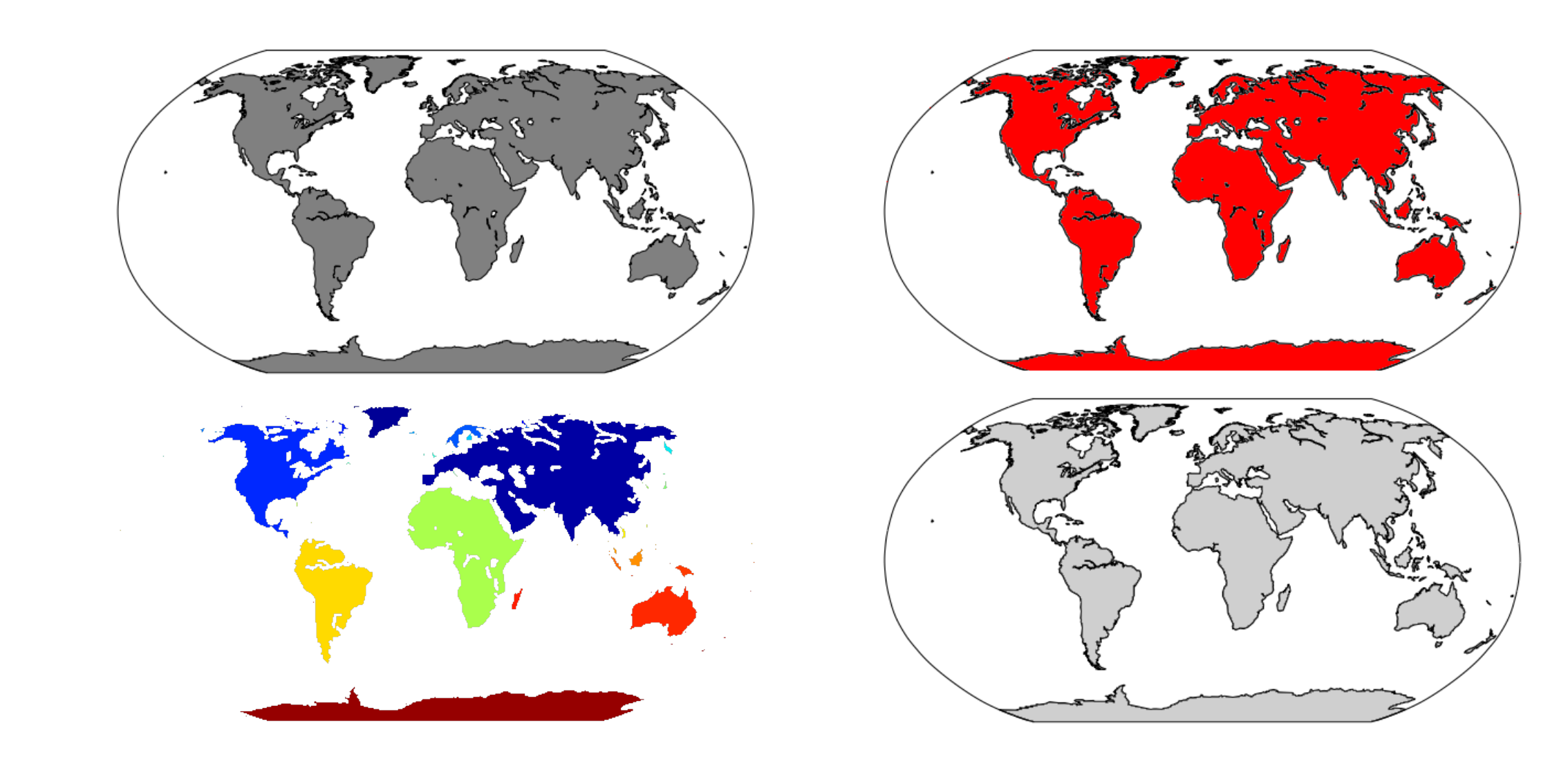
la première image est l'originale, la seconde identifie la masse terrestre. Le troisième n'est pas nécessaire, mais amusant car il ID's chacun séparé contiguous landmass. La quatrième image est ce que vous voulez, l'image avec le "rivers" enlevé.
suivant l'exemple de user1868739, Je ne peux sélectionner que les chemins (pour certains lacs) que je veux:
from mpl_toolkits.basemap import Basemap
import matplotlib.pyplot as plt

fig = plt.figure(figsize=(8, 4.5))
plt.subplots_adjust(left=0.02, right=0.98, top=0.98, bottom=0.00)
m = Basemap(resolution='c',projection='robin',lon_0=0)
m.fillcontinents(color='white',lake_color='white',zorder=2)
coasts = m.drawcoastlines(zorder=1,color='white',linewidth=0)
coasts_paths = coasts.get_paths()

ipolygons = range(83) + [84] # want Baikal, but not Tanganyika
# 80 = Superior+Michigan+Huron, 81 = Victoria, 82 = Aral, 83 = Tanganyika,
# 84 = Baikal, 85 = Great Bear, 86 = Great Slave, 87 = Nyasa, 88 = Erie
# 89 = Winnipeg, 90 = Ontario
for ipoly in ipolygons:
    r = coasts_paths[ipoly]
    # Convert into lon/lat vertices
    polygon_vertices = [(vertex[0],vertex[1]) for (vertex,code) in
                        r.iter_segments(simplify=False)]
    px = [polygon_vertices[i][0] for i in xrange(len(polygon_vertices))]
    py = [polygon_vertices[i][2] for i in xrange(len(polygon_vertices))]
    m.plot(px,py,linewidth=0.5,zorder=3,color='black')

plt.savefig('world2.png',dpi=100)
mais cela ne fonctionne qu'en utilisant le fond blanc pour les continents. Si je change d' color'gray' dans la ligne suivante, nous voyons que d'autres rivières et lacs ne sont pas remplis de la même couleur que les continents. (Aussi jouer avec area_thresh n'enlèvera pas les rivières qui sont reliées à océan.)
m.fillcontinents(color='gray',lake_color='white',zorder=2)
la version avec fond blanc est appropriée pour plus de couleur-traçant toutes sortes d'informations de terre sur les continents, mais une solution plus élaborée serait nécessaire, si l'on veut conserver le fond gris pour les continents.
je modifie fréquemment les lignes de tiroirs de Basemap() pour éviter ces rivières "cassées". Je modifie également drawcoups () par souci de cohérence des sources de données.
voici ce que j'utilise pour supporter les différentes résolutions disponibles dans les données de la Terre naturelle:
from mpl_toolkits.basemap import Basemap


class Basemap(Basemap):
    """ Modify Basemap to use Natural Earth data instead of GSHHG data """
    def drawcoastlines(self):
        shapefile = 'data/naturalearth/coastline/ne_%sm_coastline' % \
                    {'l':110, 'm':50, 'h':10}[self.resolution]
        self.readshapefile(shapefile, 'coastline', linewidth=1.)
    def drawcountries(self):
        shapefile = 'data/naturalearth/countries/ne_%sm_admin_0_countries' % \
                    {'l':110, 'm':50, 'h':10}[self.resolution]
        self.readshapefile(shapefile, 'countries', linewidth=0.5)


m = Basemap(llcrnrlon=-90, llcrnrlat=-40, urcrnrlon=-30, urcrnrlat=+20,
            resolution='l')  # resolution = (l)ow | (m)edium | (h)igh
m.drawcoastlines()
m.drawcountries()
veuillez noter que par défaut Basemap utilise resolution='c' (crude), qui n'est pas supporté dans le code affiché.
si vous êtes D'accord avec le tracé des contours plutôt que les shapefiles, il est assez facile de tracer les côtes que vous pouvez obtenir de n'importe où. J'ai eu mes côtes grâce à L'Extracteur de côte NOAA au format MATLAB.: http://www.ngdc.noaa.gov/mgg/shorelines/shorelines.html
pour éditer les littoraux, je les ai convertis en SVG, puis je les ai édités avec Inkscape, puis je les ai reconvertis dans le fichier texte lat/lon (format"MATLAB").
tout le code Python est inclus dessous.
# ---------------------------------------------------------------
def plot_lines(mymap, lons, lats, **kwargs) :
    """Plots a custom coastline.  This plots simple lines, not
    ArcInfo-style SHAPE files.

    Args:
        lons: Longitude coordinates for line segments (degrees E)
        lats: Latitude coordinates for line segments (degrees N)

    Type Info:
        len(lons) == len(lats)
        A NaN in lons and lats signifies a new line segment.

    See:
        giss.noaa.drawcoastline_file()
    """

    # Project onto the map
    x, y = mymap(lons, lats)

    # BUG workaround: Basemap projects our NaN's to 1e30.
    x[x==1e30] = np.nan
    y[y==1e30] = np.nan

    # Plot projected line segments.
    mymap.plot(x, y, **kwargs)


# Read "Matlab" format files from NOAA Coastline Extractor.
# See: http://www.ngdc.noaa.gov/mgg/coast/

lineRE=re.compile('(.*?)\s+(.*)')
def read_coastline(fname, take_every=1) :
    nlines = 0
    xdata = array.array('d')
    ydata = array.array('d')
    for line in file(fname) :
#        if (nlines % 10000 == 0) :
#            print 'nlines = %d' % (nlines,)
        if (nlines % take_every == 0 or line[0:3] == 'nan') :
            match = lineRE.match(line)
            lon = float(match.group(1))
            lat = float(match.group(2))

            xdata.append(lon)
            ydata.append(lat)
        nlines = nlines + 1


    return (np.array(xdata),np.array(ydata))

def drawcoastline_file(mymap, fname, **kwargs) :
    """Reads and plots a coastline file.
    See:
        giss.basemap.drawcoastline()
        giss.basemap.read_coastline()
    """

    lons, lats = read_coastline(fname, take_every=1)
    return drawcoastline(mymap, lons, lats, **kwargs)
# =========================================================
# coastline2svg.py
#
import giss.io.noaa
import os
import numpy as np
import sys

svg_header = """<?xml version="1.0" encoding="UTF-8" standalone="no"?>
<!-- Created with Inkscape (http://www.inkscape.org/) -->

<svg
   xmlns:dc="http://purl.org/dc/elements/1.1/"
   xmlns:cc="http://creativecommons.org/ns#"
   xmlns:rdf="http://www.w3.org/1999/02/22-rdf-syntax-ns#"
   xmlns:svg="http://www.w3.org/2000/svg"
   xmlns="http://www.w3.org/2000/svg"
   version="1.1"
   width="360"
   height="180"
   id="svg2">
  <defs
     id="defs4" />
  <metadata
     id="metadata7">
    <rdf:RDF>
      <cc:Work
         rdf:about="">
        <dc:format>image/svg+xml</dc:format>
        <dc:type
           rdf:resource="http://purl.org/dc/dcmitype/StillImage" />
        <dc:title></dc:title>
      </cc:Work>
    </rdf:RDF>
  </metadata>
  <g
     id="layer1">
"""

path_tpl = """
    <path
       d="%PATH%"
       id="%PATH_ID%"
       style="fill:none;stroke:#000000;stroke-width:1px;stroke-linecap:butt;stroke-linejoin:miter;stroke-opacity:1"
"""

svg_footer = "</g></svg>"


# Set up paths
data_root = os.path.join(os.environ['HOME'], 'data')
#modelerc = giss.modele.read_modelerc()
#cmrun = modelerc['CMRUNDIR']
#savedisk = modelerc['SAVEDISK']

ifname = sys.argv[1]
ofname = ifname.replace('.dat', '.svg')

lons, lats = giss.io.noaa.read_coastline(ifname, 1)

out = open(ofname, 'w')
out.write(svg_header)

path_id = 1
points = []
for lon, lat in zip(lons, lats) :
    if np.isnan(lon) or np.isnan(lat) :
        # Process what we have
        if len(points) > 2 :
            out.write('\n<path d="')
            out.write('m %f,%f L' % (points[0][0], points[0][1]))
            for pt in points[1:] :
                out.write(' %f,%f' % pt)
            out.write('"\n   id="path%d"\n' % (path_id))
#            out.write('style="fill:none;stroke:#000000;stroke-width:1px;stroke-linecap:butt;stroke-linejoin:miter;stroke-opacity:1"')
            out.write(' />\n')
            path_id += 1
        points = []
    else :
        lon += 180
        lat = 180 - (lat + 90)
        points.append((lon, lat))


out.write(svg_footer)
out.close()

# =============================================================
# svg2coastline.py

import os
import sys
import re

# Reads the output of Inkscape's "Plain SVG" format, outputs in NOAA MATLAB coastline format

mainRE = re.compile(r'\s*d=".*"')
lineRE = re.compile(r'\s*d="(m|M)\s*(.*?)"')

fname = sys.argv[1]


lons = []
lats = []
for line in open(fname, 'r') :
    # Weed out extraneous lines in the SVG file
    match = mainRE.match(line)
    if match is None :
        continue

    match = lineRE.match(line)

    # Stop if something is wrong
    if match is None :
        sys.stderr.write(line)
        sys.exit(-1)

    type = match.group(1)[0]
    spairs = match.group(2).split(' ')
    x = 0
    y = 0
    for spair in spairs :
        if spair == 'L' :
            type = 'M'
            continue

        (sdelx, sdely) = spair.split(',')
        delx = float(sdelx)
        dely = float(sdely)
        if type == 'm' :
            x += delx
            y += dely
        else :
            x = delx
            y = dely
        lon = x - 180
        lat = 90 - y
        print '%f\t%f' % (lon, lat)
    print 'nan\tnan'
l'idée de base est que les chemins utilisés par drawcoastlines() sont ordonnés par la taille/zone. Ce qui signifie que les premiers n sentiers sont (pour la plupart des applications) les masses terrestres principales et les lacs et les sentiers plus tard, les îles plus petites et les rivières.
le problème est que les N premières voies que vous voulez dépendra de la projection (par exemple, globale, polaire, régionale), si area_thresh a été appliqué et si vous voulez des lacs ou petits îles etc. En d'autres termes, vous devrez modifier ceci par application.
from mpl_toolkits.basemap import Basemap
import matplotlib.pyplot as plt

mp = 'cyl'
m = Basemap(resolution='c',projection=mp,lon_0=0,area_thresh=200000)

fill_color = '0.9'

# If you don't want lakes set lake_color to fill_color
m.fillcontinents(color=fill_color,lake_color='white')

# Draw the coastlines, with a thin line and same color as the continent fill.
coasts = m.drawcoastlines(zorder=100,color=fill_color,linewidth=0.5)

# Exact the paths from coasts
coasts_paths = coasts.get_paths()

# In order to see which paths you want to retain or discard you'll need to plot them one
# at a time noting those that you want etc.
for ipoly in xrange(len(coasts_paths)):
    print ipoly
    r = coasts_paths[ipoly]
    # Convert into lon/lat vertices
    polygon_vertices = [(vertex[0],vertex[1]) for (vertex,code) in
                        r.iter_segments(simplify=False)]
    px = [polygon_vertices[i][0] for i in xrange(len(polygon_vertices))]
    py = [polygon_vertices[i][1] for i in xrange(len(polygon_vertices))]
    m.plot(px,py,'k-',linewidth=1)
    plt.show()
une fois que vous connaissez l'ipoly appropriée pour arrêter le dessin (poly_stop) alors vous pouvez faire quelque chose comme ça...
from mpl_toolkits.basemap import Basemap
import matplotlib.pyplot as plt

mproj = ['nplaea','cyl']
mp = mproj[0]

if mp == 'nplaea':
    m = Basemap(resolution='c',projection=mp,lon_0=0,boundinglat=30,area_thresh=200000,round=1)
    poly_stop = 10
else:
    m = Basemap(resolution='c',projection=mp,lon_0=0,area_thresh=200000)
    poly_stop = 18
fill_color = '0.9'

# If you don't want lakes set lake_color to fill_color
m.fillcontinents(color=fill_color,lake_color='white')

# Draw the coastlines, with a thin line and same color as the continent fill.
coasts = m.drawcoastlines(zorder=100,color=fill_color,linewidth=0.5)

# Exact the paths from coasts
coasts_paths = coasts.get_paths()

# In order to see which paths you want to retain or discard you'll need to plot them one
# at a time noting those that you want etc.
for ipoly in xrange(len(coasts_paths)):
    if ipoly > poly_stop: continue
    r = coasts_paths[ipoly]
    # Convert into lon/lat vertices
    polygon_vertices = [(vertex[0],vertex[1]) for (vertex,code) in
                        r.iter_segments(simplify=False)]
    px = [polygon_vertices[i][0] for i in xrange(len(polygon_vertices))]
    py = [polygon_vertices[i][1] for i in xrange(len(polygon_vertices))]
    m.plot(px,py,'k-',linewidth=1)
plt.show()
selon mon commentaire à @sampo-smolander
from mpl_toolkits.basemap import Basemap
import matplotlib.pyplot as plt

fig = plt.figure(figsize=(8, 4.5))
plt.subplots_adjust(left=0.02, right=0.98, top=0.98, bottom=0.00)
m = Basemap(resolution='c',projection='robin',lon_0=0)
m.fillcontinents(color='gray',lake_color='white',zorder=2)
coasts = m.drawcoastlines(zorder=1,color='white',linewidth=0)
coasts_paths = coasts.get_paths()

ipolygons = range(83) + [84]
for ipoly in xrange(len(coasts_paths)):
    r = coasts_paths[ipoly]
    # Convert into lon/lat vertices
    polygon_vertices = [(vertex[0],vertex[1]) for (vertex,code) in
                        r.iter_segments(simplify=False)]
    px = [polygon_vertices[i][0] for i in xrange(len(polygon_vertices))]
    py = [polygon_vertices[i][1] for i in xrange(len(polygon_vertices))]
    if ipoly in ipolygons:
        m.plot(px,py,linewidth=0.5,zorder=3,color='black')
    else:
        m.plot(px,py,linewidth=0.5,zorder=4,color='grey')
plt.savefig('world2.png',dpi=100)
