R points de superposition et polygones présentant un certain degré de tolérance
en utilisant R, j'aimerais superposer quelques points spatiaux et polygones afin d'attribuer aux points quelques attributs des régions géographiques que j'ai prises en considération.
ce que je fais habituellement est d'utiliser la commande oversp paquet. Mes problèmes sont que je travaille avec un grand nombre d'événements géoréférencés qui se sont produits partout dans le monde et dans certains cas (en particulier dans les zones côtières), la combinaison longitude et latitude tombe légèrement en dehors de la pays/région frontière.
Voici un exemple reproductible basé sur ce très bonne question.
## example data
set.seed(1)
library(raster)
library(rgdal)
library(sp)
p <- shapefile(system.file("external/lux.shp", package="raster"))
p2 <- as(0.30*extent(p), "SpatialPolygons")
proj4string(p2) <- proj4string(p)
pts1 <- spsample(p2-p, n=3, type="random")
pts2<- spsample(p, n=10, type="random")
pts<-rbind(pts1, pts2)
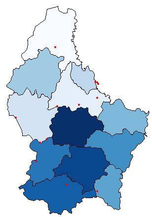
## Plot to visualize
plot(p, col=colorRampPalette(blues9)(12))
plot(pts, pch=16, cex=.5,col="red", add=TRUE)
# overlay
pts_index<-over(pts, p)

# result
pts_index

#>     ID_1       NAME_1 ID_2           NAME_2 AREA
#>1    NA         <NA> <NA>             <NA>   NA
#>2    NA         <NA> <NA>             <NA>   NA
#>3    NA         <NA> <NA>             <NA>   NA
#>4     1     Diekirch    1         Clervaux  312
#>5     1     Diekirch    5            Wiltz  263
#>6     2 Grevenmacher   12     Grevenmacher  210
#>7     2 Grevenmacher    6       Echternach  188
#>8     3   Luxembourg    9 Esch-sur-Alzette  251
#>9     1     Diekirch    3          Redange  259
#>10    2 Grevenmacher    7           Remich  129
#>11    1     Diekirch    1         Clervaux  312
#>12    1     Diekirch    5            Wiltz  263
#>13    2 Grevenmacher    7           Remich  129
Est-il possible de donner à l' over fonction d'une sorte de tolérance, afin de saisir également les points qui sont très proche de la frontière?
NOTE:
Suivant je pourrais assigner au point manquant le polygone le plus proche, mais ce n'est pas exactement ce que je suis après.
EDIT: near neighbor solution
#adding lon and lat to the table
pts_index$lon<-pts@coords[,1]
pts_index$lat<-pts@coords[,2]

#add an ID to split and then re-compose the table
pts_index$split_id<-seq(1,nrow(pts_index),1)
#filtering out the missed points

library(dplyr)
library(geosphere)
missed_pts<-filter(pts_index, is.na(NAME_1))
pts_missed<-SpatialPoints(missed_pts[,c(6,7)],proj4string=CRS(proj4string(p)))

#find the nearest neighbors' characteristics
n <- length(pts_missed)
nearestID1 <- character(n)
nearestNAME1 <- character(n)
nearestID2 <- character(n)
nearestNAME2 <- character(n)
nearestAREA <- character(n)

for (i in seq_along(nearestID1)) {
  nearestID1[i] <- as.character(p$ID_1[which.min(dist2Line (pts_missed[i,], p))])
  nearestNAME1[i] <- as.character(p$NAME_1[which.min(dist2Line (pts_missed[i,], p))])
  nearestID2[i] <- as.character(p$ID_2[which.min(dist2Line (pts_missed[i,], p))])
  nearestNAME2[i] <- as.character(p$NAME_2[which.min(dist2Line (pts_missed[i,], p))])
  nearestAREA[i] <- as.character(p$AREA[which.min(dist2Line (pts_missed[i,], p))])
}
missed_pts$ID_1<-nearestID1
missed_pts$NAME_1<-nearestNAME1
missed_pts$ID_2<-nearestID2
missed_pts$NAME_2<-nearestNAME2
missed_pts$AREA<-nearestAREA

#missed_pts have now the characteristics of the nearest poliygon
#bringing now everything toogether
pts_index[match(missed_pts$split_id, pts_index$split_id),] <- missed_pts
pts_index<-pts_index[,-c(6:8)]

pts_index

       ID_1       NAME_1 ID_2           NAME_2 AREA
1     1     Diekirch    4          Vianden   76
2     1     Diekirch    4          Vianden   76
3     1     Diekirch    4          Vianden   76
4     1     Diekirch    1         Clervaux  312
5     1     Diekirch    5            Wiltz  263
6     2 Grevenmacher   12     Grevenmacher  210
7     2 Grevenmacher    6       Echternach  188
8     3   Luxembourg    9 Esch-sur-Alzette  251
9     1     Diekirch    3          Redange  259
10    2 Grevenmacher    7           Remich  129
11    1     Diekirch    1         Clervaux  312
12    1     Diekirch    5            Wiltz  263
13    2 Grevenmacher    7           Remich  129
C'est exactement le même résultat que celui proposé par @Gilles dans sa réponse. Je me demande juste s'il y a quelque chose de plus efficace que tout ça.
3 réponses
L'exemple de données
set.seed(1)
library(raster)
library(rgdal)
library(sp)
p <- shapefile(system.file("external/lux.shp", package="raster"))
p2 <- as(0.30*extent(p), "SpatialPolygons")
proj4string(p2) <- proj4string(p)
pts1 <- spsample(p2-p, n=3, type="random")
pts2<- spsample(p, n=10, type="random")
pts<-rbind(pts1, pts2)

## Plot to visualize
plot(p, col=colorRampPalette(blues9)(12))
plot(pts, pch=16, cex=.5,col="red", add=TRUE)
Solution en utilisant sf et nngeo paquets
library(nngeo)

# Convert to 'sf'
pts = st_as_sf(pts)
p = st_as_sf(p)

# Spatial join
p1 = st_join(pts, p, join = st_nn)
p1

## Simple feature collection with 13 features and 5 fields
## geometry type:  POINT
## dimension:      XY
## bbox:           xmin: 5.795068 ymin: 49.54622 xmax: 6.518138 ymax: 50.1426
## epsg (SRID):    4326
## proj4string:    +proj=longlat +datum=WGS84 +no_defs
## First 10 features:
##   ID_1       NAME_1 ID_2           NAME_2 AREA                  geometry
## 1     1     Diekirch    4          Vianden   76 POINT (6.235953 49.91801)
## 2     1     Diekirch    4          Vianden   76 POINT (6.251893 49.92177)
## 3     1     Diekirch    4          Vianden   76  POINT (6.236712 49.9023)
## 4     1     Diekirch    1         Clervaux  312  POINT (6.090294 50.1426)
## 5     1     Diekirch    5            Wiltz  263  POINT (5.948738 49.8796)
## 6     2 Grevenmacher   12     Grevenmacher  210 POINT (6.302851 49.66278)
## 7     2 Grevenmacher    6       Echternach  188 POINT (6.518138 49.76773)
## 8     3   Luxembourg    9 Esch-sur-Alzette  251 POINT (6.116905 49.56184)
## 9     1     Diekirch    3          Redange  259 POINT (5.932418 49.78505)
## 10    2 Grevenmacher    7           Remich  129 POINT (6.285379 49.54622)
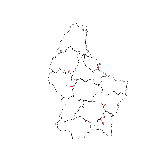
graphe montrant quels polygones et points sont reliés -
# Visuzlize join
l = st_connect(pts, p, dist = 1)
plot(st_geometry(p))
plot(st_geometry(pts), add = TRUE)
plot(st_geometry(l), col = "red", lwd = 2, add = TRUE)
EDIT:
# Spatial join with 100 meters threshold
p2 = st_join(pts, p, join = st_nn, maxdist = 100)
p2
## Simple feature collection with 13 features and 5 fields
## geometry type:  POINT
## dimension:      XY
## bbox:           xmin: 5.795068 ymin: 49.54622 xmax: 6.518138 ymax: 50.1426
## epsg (SRID):    4326
## proj4string:    +proj=longlat +datum=WGS84 +no_defs
## First 10 features:
##   ID_1       NAME_1 ID_2           NAME_2 AREA                  geometry
## 1    NA         <NA> <NA>             <NA>   NA POINT (6.235953 49.91801)
## 2    NA         <NA> <NA>             <NA>   NA POINT (6.251893 49.92177)
## 3     1     Diekirch    4          Vianden   76  POINT (6.236712 49.9023)
## 4     1     Diekirch    1         Clervaux  312  POINT (6.090294 50.1426)
## 5     1     Diekirch    5            Wiltz  263  POINT (5.948738 49.8796)
## 6     2 Grevenmacher   12     Grevenmacher  210 POINT (6.302851 49.66278)
## 7     2 Grevenmacher    6       Echternach  188 POINT (6.518138 49.76773)
## 8     3   Luxembourg    9 Esch-sur-Alzette  251 POINT (6.116905 49.56184)
## 9     1     Diekirch    3          Redange  259 POINT (5.932418 49.78505)
## 10    2 Grevenmacher    7           Remich  129 POINT (6.285379 49.54622)
Voici ma tentative à l'aide de sf. Dans le cas où vous voulez aveuglément joindre des traits de polygone pour former des points leur plus proche voisin, il suffit d'appeler st_joinjoin = st_nearest_feature
library(sf)

# convert data to sf
pts_sf = st_as_sf(pts)
p_sf = st_as_sf(p)

# this is enough for joining polygon attributes to points from their nearest neighbor
st_join(pts_sf, p_sf, join = st_nearest_feature)
si vous voulez être en mesure de définir une certaine tolérance de sorte que les points plus éloignés que cette tolérance n'obtiendront pas d'attributs polygonaux joints, nous devons créer notre propre fonction jointure.
st_nearest_feature2 = function(x, y, tolerance = 100) {
  isec = st_intersects(x, y)
  no_isec = which(lengths(isec) == 0)

  for (i in no_isec) {
    nrst = st_nearest_points(st_geometry(x)[i], y)
    nrst_len = st_length(nrst)
    nrst_mn = which.min(nrst_len)
    isec[i] = ifelse(as.vector(nrst_len[nrst_mn]) > tolerance, integer(0), nrst_mn)
  }

  unlist(isec)

}

st_join(pts_sf, p_sf, join = st_nearest_feature2, tolerance = 1000)
cela fonctionne comme prévu, i.e. quand vous définissez tolerance à zéro, vous obtiendrez la même résultat en plus et pour des valeurs plus grandes vous approcherez le st_nearest_feature résultat d'en haut.
je ne pense pas que vous pouvez ajouter une "tolérance" à l' over ou d'autres algorithmes d'intersection.
En tamponnant les polygones, vous ajouteriez une certaine tolérance, mais alors certains points pourraient tomber dans deux polygones différents.
une possibilité pourrait être de créer une zone tampon autour des points qui se situent à l'extérieur des polygones de régions, de croiser ces zones tampons avec les polygones, de calculer la zone et pour chaque point de garder seulement les lignes avec la zone maximale. L'avantage de cette approche par rapport à celui que vous suggérez (trouver le plus proche polygone), c'est que vous n'avez pas à calculer la distance avec tous les polygones.
il y a probablement des possibilités plus directes...
Voici un exemple d'utilisation sf pour manipuler les objets géographiques, mais vous pouvez certainement faire de même avec sp et rgeos.
Une difficulté est de trouver le bon niveau de "tolérance" (Taille du tampon). J'utilise ici une tolérance de 2km.
## Your example
set.seed(1)
library(raster)
#> Loading required package: sp
library(rgdal)
library(sp)


p <- shapefile(system.file("external/lux.shp", package="raster"))
p2 <- as(0.30*extent(p), "SpatialPolygons")
proj4string(p2) <- proj4string(p)
pts1 <- spsample(p2-p, n=3, type="random")
pts2<- spsample(p, n=10, type="random")
pts<-rbind(pts1, pts2)
Notez que je n'ai pas la même sortie que vous over:
over(pts, p)
#>    ID_1       NAME_1 ID_2           NAME_2 AREA
#> 1    NA         <NA> <NA>             <NA>   NA
#> 2    NA         <NA> <NA>             <NA>   NA
#> 3    NA         <NA> <NA>             <NA>   NA
#> 4     1     Diekirch    1         Clervaux  312
#> 5     1     Diekirch    5            Wiltz  263
#> 6     2 Grevenmacher   12     Grevenmacher  210
#> 7     2 Grevenmacher    6       Echternach  188
#> 8     3   Luxembourg    9 Esch-sur-Alzette  251
#> 9     1     Diekirch    3          Redange  259
#> 10    2 Grevenmacher    7           Remich  129
#> 11    1     Diekirch    1         Clervaux  312
#> 12    1     Diekirch    5            Wiltz  263
#> 13    2 Grevenmacher    7           Remich  129
utilisant des tampons sur les points qui se situent à l'extérieur des polygones:
# additional packages needed
library(sf)
library(dplyr)

# transform the sp objects into sf objects and add an ID to the points
pts <- st_as_sf(pts)
pts$IDpts <- 1:nrow(pts)
p <- st_as_sf(p)

# project the data in planar coordinates (here a projection for Luxemburg)
# better for area calculations but maybe not crucial here
pts <- st_transform(pts, crs = 2169)
p <- st_transform(p, crs = 2169)


# intersect the points with the polygons (equivalent to you "over")
pts_index <- st_set_geometry(st_intersection(pts, p), NULL)
#> Warning: attribute variables are assumed to be spatially constant
#> throughout all geometries


# points that are outside the polygons
pts_out <- pts[lengths(st_within(pts, p)) == 0,]
# buffer around these points with a given size
bf <- st_buffer(pts_out, dist = 2000) # distance in meters, here 2km

# intersect these buffers with the polygons and compute their area
bf <- st_intersection(bf, p)
#> Warning: attribute variables are assumed to be spatially constant
#> throughout all geometries
bf$area <- st_area(bf)

# for each point (IDpts), select the line with the highest area
# then drop the geometry columns and transform the result n a data.frame
pts_out <- bf %>% group_by(IDpts) %>% slice(which.max(area)) %>%
     select(1:6) %>% st_set_geometry(NULL) %>% as.data.frame()
Sortie :
# Colate the results from the point within polygons and outside polygons
pts_index <- rbind(pts_index, pts_out)
pts_index <- pts_index[order(pts_index$IDpts),]
pts_index
#>    IDpts ID_1       NAME_1 ID_2           NAME_2 AREA
#> 1      1    1     Diekirch    4          Vianden   76
#> 2      2    1     Diekirch    4          Vianden   76
#> 3      3    1     Diekirch    4          Vianden   76
#> 4      4    1     Diekirch    1         Clervaux  312
#> 5      5    1     Diekirch    5            Wiltz  263
#> 6      6    2 Grevenmacher   12     Grevenmacher  210
#> 7      7    2 Grevenmacher    6       Echternach  188
#> 8      8    3   Luxembourg    9 Esch-sur-Alzette  251
#> 9      9    1     Diekirch    3          Redange  259
#> 10    10    2 Grevenmacher    7           Remich  129
#> 11    11    1     Diekirch    1         Clervaux  312
#> 12    12    1     Diekirch    5            Wiltz  263
#> 13    13    2 Grevenmacher    7           Remich  129