Comment tracer une carte 3D de la densité en python avec matplotlib
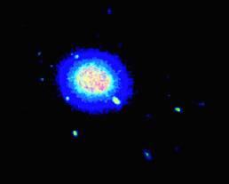
j'ai un grand ensemble de données de (x,y,z) positions de protéines et je voudrais tracer les zones d'occupation élevée comme une heatmap. Idéalement, la sortie devrait ressembler à la visualisation volumétrique ci-dessous, mais je ne suis pas sûr de la façon d'y parvenir avec matplotlib.
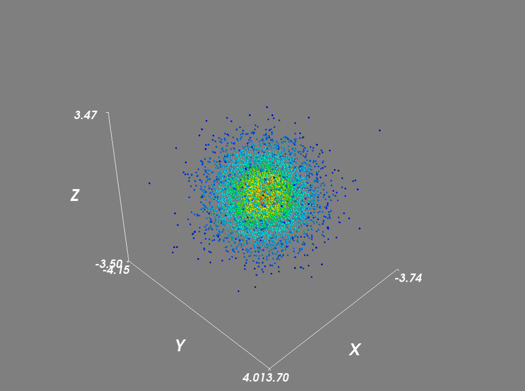
mon idée initiale était d'afficher mes positions comme un nuage de points 3D et de colorer leur densité via un KDE. J'ai codé ceci comme suit avec test données:
import numpy as np
from scipy import stats
import matplotlib.pyplot as plt
from mpl_toolkits.mplot3d import Axes3D

mu, sigma = 0, 0.1
x = np.random.normal(mu, sigma, 1000)
y = np.random.normal(mu, sigma, 1000)
z = np.random.normal(mu, sigma, 1000)

xyz = np.vstack([x,y,z])
density = stats.gaussian_kde(xyz)(xyz)

idx = density.argsort()
x, y, z, density = x[idx], y[idx], z[idx], density[idx]

fig = plt.figure()
ax = fig.add_subplot(111, projection='3d')
ax.scatter(x, y, z, c=density)
plt.show()
Cela fonctionne bien! Cependant, mes données réelles contiennent des milliers de points de données et le calcul du kde et du scatter plot devient extrêmement lent.
<!-Un petit échantillon de mes données réelles: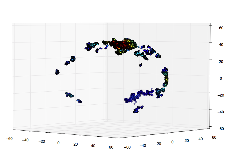
Mes recherches suggèrent qu'une meilleure option est d'évaluer la gaussienne kde sur une grille. Je ne sais pas comment faire en 3D:
import numpy as np
from scipy import stats
import matplotlib.pyplot as plt
from mpl_toolkits.mplot3d import Axes3D

mu, sigma = 0, 0.1
x = np.random.normal(mu, sigma, 1000)
y = np.random.normal(mu, sigma, 1000)

nbins = 50

xy = np.vstack([x,y])
density = stats.gaussian_kde(xy)

xi, yi = np.mgrid[x.min():x.max():nbins*1j, y.min():y.max():nbins*1j]
di = density(np.vstack([xi.flatten(), yi.flatten()]))

fig = plt.figure()
ax = fig.add_subplot(111)
ax.pcolormesh(xi, yi, di.reshape(xi.shape))
plt.show()
1 réponses
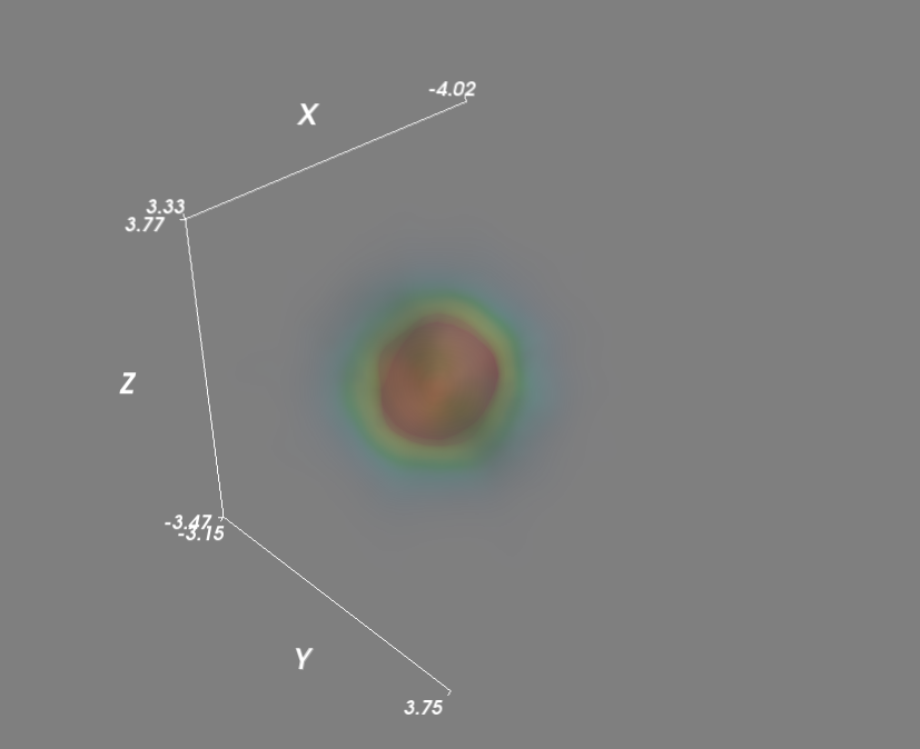
merci à mwaskon d'avoir suggéré la bibliothèque mayavi.
j'ai recréé le diagramme de dispersion de la densité à mayavi comme suit:
import numpy as np
from scipy import stats
from mayavi import mlab

mu, sigma = 0, 0.1
x = 10*np.random.normal(mu, sigma, 5000)
y = 10*np.random.normal(mu, sigma, 5000)
z = 10*np.random.normal(mu, sigma, 5000)

xyz = np.vstack([x,y,z])
kde = stats.gaussian_kde(xyz)
density = kde(xyz)

# Plot scatter with mayavi
figure = mlab.figure('DensityPlot')
pts = mlab.points3d(x, y, z, density, scale_mode='none', scale_factor=0.07)
mlab.axes()
mlab.show()
paramétrer le scale_mode à 'none' empêche glyphs d'être mis à l'échelle en proportion du vecteur de densité. En outre pour les grands ensembles de données, j'ai désactivé le rendu de scène et utilisé un masque pour réduire le nombre de points.
# Plot scatter with mayavi
figure = mlab.figure('DensityPlot')
figure.scene.disable_render = True

pts = mlab.points3d(x, y, z, density, scale_mode='none', scale_factor=0.07)
mask = pts.glyph.mask_points
mask.maximum_number_of_points = x.size
mask.on_ratio = 1
pts.glyph.mask_input_points = True

figure.scene.disable_render = False
mlab.axes()
mlab.show()
ensuite, évaluer le KDE gaussien sur un grille:
import numpy as np
from scipy import stats
from mayavi import mlab

mu, sigma = 0, 0.1
x = 10*np.random.normal(mu, sigma, 5000)
y = 10*np.random.normal(mu, sigma, 5000)
z = 10*np.random.normal(mu, sigma, 5000)

xyz = np.vstack([x,y,z])
kde = stats.gaussian_kde(xyz)

# Evaluate kde on a grid
xmin, ymin, zmin = x.min(), y.min(), z.min()
xmax, ymax, zmax = x.max(), y.max(), z.max()
xi, yi, zi = np.mgrid[xmin:xmax:30j, ymin:ymax:30j, zmin:zmax:30j]
coords = np.vstack([item.ravel() for item in [xi, yi, zi]])
density = kde(coords).reshape(xi.shape)

# Plot scatter with mayavi
figure = mlab.figure('DensityPlot')

grid = mlab.pipeline.scalar_field(xi, yi, zi, density)
min = density.min()
max=density.max()
mlab.pipeline.volume(grid, vmin=min, vmax=min + .5*(max-min))

mlab.axes()
mlab.show()
import numpy as np
from scipy import stats
from mayavi import mlab
import multiprocessing

def calc_kde(data):
    return kde(data.T)

mu, sigma = 0, 0.1
x = 10*np.random.normal(mu, sigma, 5000)
y = 10*np.random.normal(mu, sigma, 5000)
z = 10*np.random.normal(mu, sigma, 5000)

xyz = np.vstack([x,y,z])
kde = stats.gaussian_kde(xyz)

# Evaluate kde on a grid
xmin, ymin, zmin = x.min(), y.min(), z.min()
xmax, ymax, zmax = x.max(), y.max(), z.max()
xi, yi, zi = np.mgrid[xmin:xmax:30j, ymin:ymax:30j, zmin:zmax:30j]
coords = np.vstack([item.ravel() for item in [xi, yi, zi]])

# Multiprocessing
cores = multiprocessing.cpu_count()
pool = multiprocessing.Pool(processes=cores)
results = pool.map(calc_kde, np.array_split(coords.T, 2))
density = np.concatenate(results).reshape(xi.shape)

# Plot scatter with mayavi
figure = mlab.figure('DensityPlot')

grid = mlab.pipeline.scalar_field(xi, yi, zi, density)
min = density.min()
max=density.max()
mlab.pipeline.volume(grid, vmin=min, vmax=min + .5*(max-min))

mlab.axes()
mlab.show()