Comment dessiner une boule de cristal avec deux couleurs de particules à l'intérieur
je lance juste une idée avec possibilité de fermeture. Je dois dessiner une boule de cristal dans laquelle les particules rouges et bleues se localisent au hasard. Je suppose que je dois aller avec photoshop, et même essayé de faire la balle dans une image, mais comme c'est pour le papier de recherche et ne doit pas être Fantaisie, je me demande s'il ya un moyen de programmer avec R, matlab, ou tout autre langage.
9 réponses
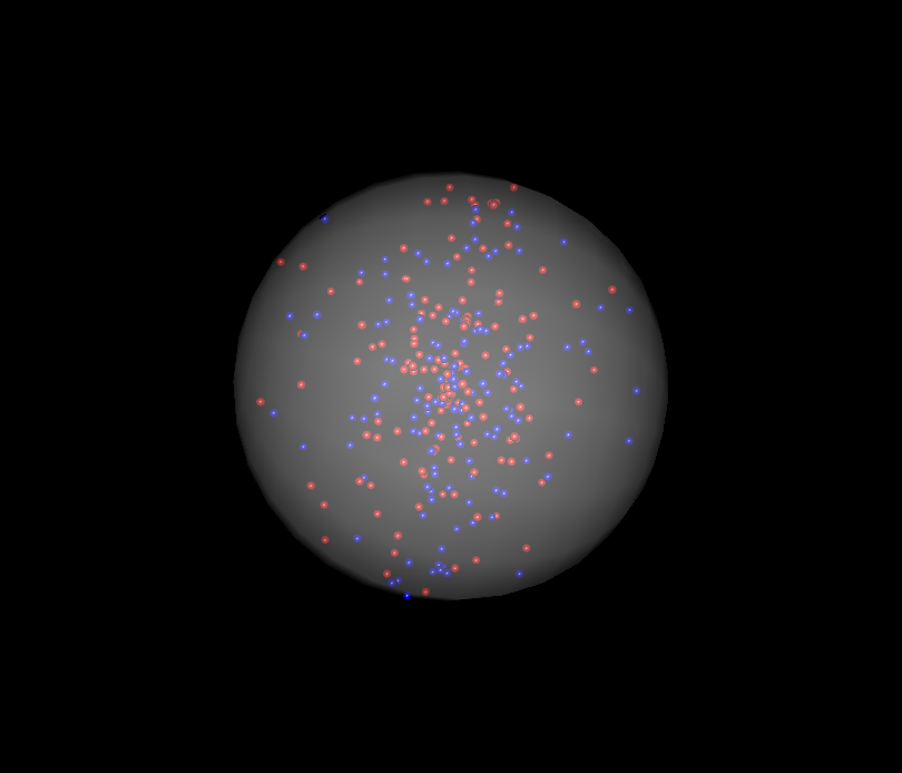
dans R, en utilisant le paquet rgl (interface R-à-OpenGL):
library(rgl)
n <- 100
set.seed(101)
randcoord <- function(n=100,r=1) {
    d <- data.frame(rho=runif(n)*r,phi=runif(n)*2*pi,psi=runif(n)*2*pi)
    with(d,data.frame(x=rho*sin(phi)*cos(psi),
                      y=rho*sin(phi)*sin(psi),
                      z=rho*cos(phi)))
}
    ## http://en.wikipedia.org/wiki/List_of_common_coordinate_transformations
with(randcoord(50,r=0.95),spheres3d(x,y,z,radius=0.02,col="red"))
with(randcoord(50,r=0.95),spheres3d(x,y,z,radius=0.02,col="blue"))
spheres3d(0,0,0,radius=1,col="white",alpha=0.5,shininess=128)
rgl.bg(col="black")
rgl.snapshot("crystalball.png")
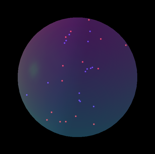
c'est très similaire à la réponse de Ben Bolker, mais je montre comment on peut ajouter un peu d'aura à la boule de cristal en utilisant une coloration mystique:
library(rgl)
lapply(seq(0.01, 1, by=0.01), function(x) rgl.spheres(0,0,0, rad=1.1*x, alpha=.01,
    col=colorRampPalette(c("orange","blue"))(100)[100*x]))
rgl.spheres(0,0,0, radius=1.11, col="red", alpha=.1)
rgl.spheres(0,0,0, radius=1.12, col="black", alpha=.1)
rgl.spheres(0,0,0, radius=1.13, col="white", alpha=.1)

xyz <- matrix(rnorm(3*100), ncol=3)
xyz <- xyz * runif(100)^(1/3) / sqrt(rowSums(xyz^2))

rgl.spheres(xyz[1:50,], rad=.02, col="blue")
rgl.spheres(xyz[51:100,], rad=.02, col="red")

rgl.bg(col="black")
rgl.viewpoint(zoom=.75)
rgl.snapshot("crystalball.png")
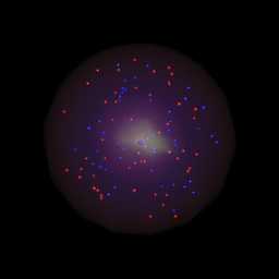
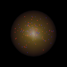
la seule différence entre les deux est dans l'appel lapply . Vous pouvez voir que juste en changeant les couleurs dans colorRampPalette vous pouvez changer l'apparence de la boule de cristal de manière significative. L'un sur l' left utilise le code lapply ci-dessus, celui de droite utilise à la place:
lapply(seq(0.01, 1, by=0.01), function(x) rgl.spheres(0,0,0,rad=1.1*x, alpha=.01,
     col=colorRampPalette(c("orange","yellow"))(100)[100*x]))
...code from above
Voici une approche différente où vous pouvez définir votre propre fichier de texture et utiliser cela pour colorer la boule de cristal:
# create a texture file, get as creative as you want:
png("texture.png")
x <- seq(1,870)
y <- seq(1,610)
z <- matrix(rnorm(870*610), nrow=870)
z <- t(apply(z,1,cumsum))/100

# Swirly texture options:
# Use the Simon O'Hanlon's roll function from this answer:
# /q/equivalent-to-numpy-roll-in-r-74046/"cyan","black"))(100), axes = FALSE)
dev.off()

xyz <- matrix(rnorm(3*100), ncol=3)
xyz <- xyz * runif(100)^(1/3) / sqrt(rowSums(xyz^2))

rgl.spheres(xyz[1:50,], rad=.02, col="blue")
rgl.spheres(xyz[51:100,], rad=.02, col="red")

rgl.spheres(0,0,0, rad=1.1, texture="texture.png", alpha=0.4, back="cull")
rgl.viewpoint(phi=90, zoom=.75) # change the view if need be
rgl.bg(color="black")
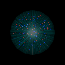
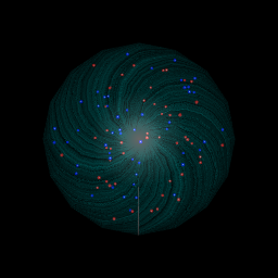 !
! 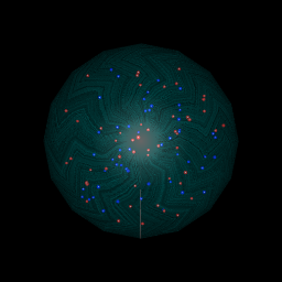
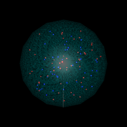
la première image en haut à gauche est ce que vous obtenez si vous exécutez le code ci-dessus, les trois autres sont les résultats de l'utilisation des différentes options dans le code de sortie commenté.
comme la question Est
je me demande s'il y a un moyen de programmer avec R, matlab, ou toute autre langue .
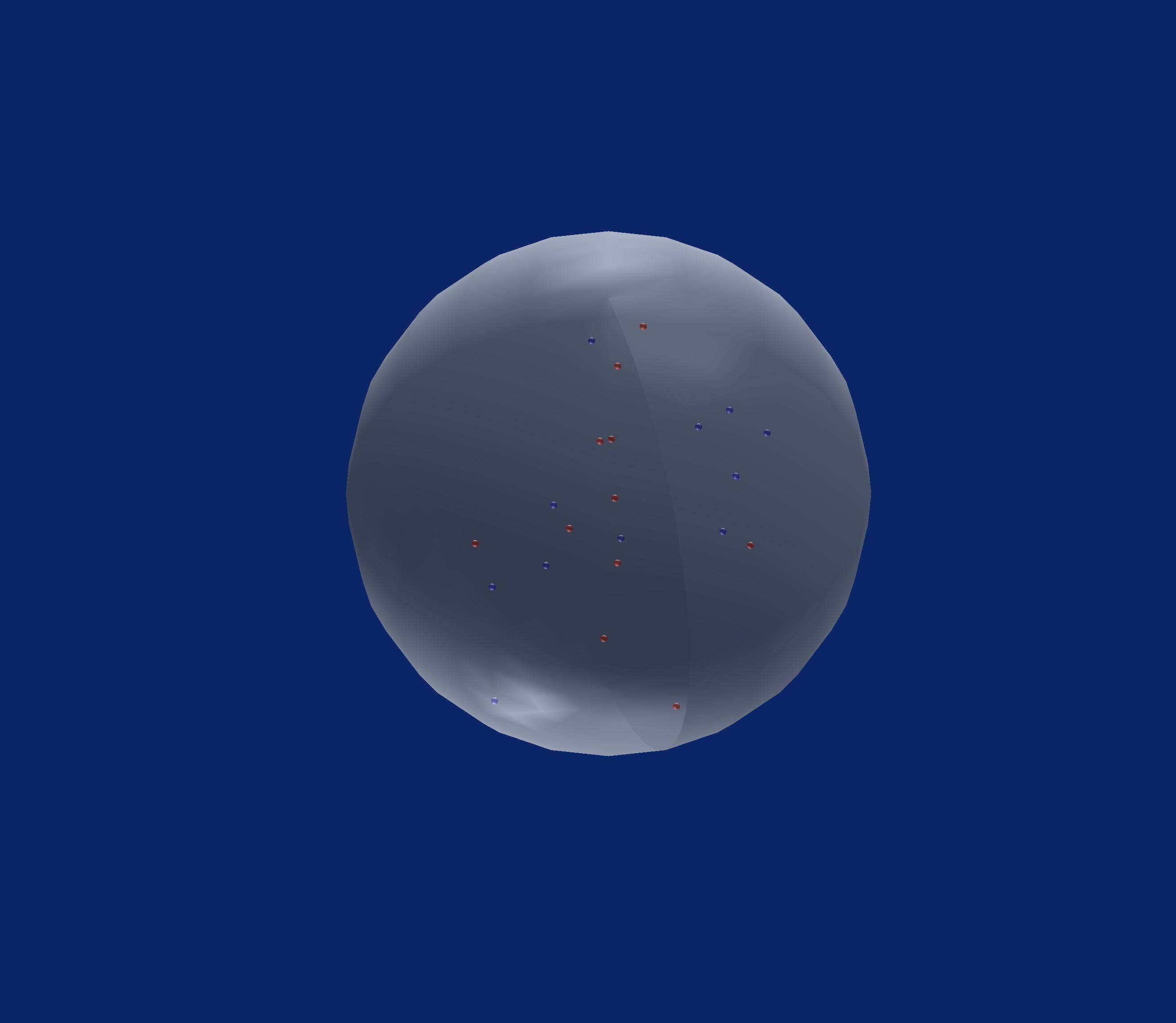
et TeX est Turing complet et peut être considéré comme un langage de programmation, j'ai pris un certain temps et créé un exemple en LaTeX en utilisant TikZ. Comme l'OP écrit c'est pour un document de recherche, cela vient avec l'avantage qu'il peut être directement intégré dans le papier, en supposant que c'est aussi écrit en LaTeX.
alors, voilà:
\documentclass[tikz]{standalone}
\usetikzlibrary{positioning, backgrounds}
\usepackage{pgf}
\pgfmathsetseed{\number\pdfrandomseed}

\begin{document}
\begin{tikzpicture}[background rectangle/.style={fill=black},
                    show background rectangle,
                   ]

    % Definitions
    \def\ballRadius{5}
    \def\pointRadius{0.1}
    \def\nRed{30}
    \def\nBlue{30}

    % Draw all red points
    \foreach \i in {1,...,\nRed}
    {
        % Get random coordinates
        \pgfmathparse{0.9*\ballRadius*rand}\let\mrho\pgfmathresult
        \pgfmathparse{360*rand}\let\mpsi\pgfmathresult
        \pgfmathparse{360*rand}\let\mphi\pgfmathresult

        % Convert to x/y/z
        \pgfmathparse{\mrho*sin(\mphi)*cos(\mpsi)}\let\mx\pgfmathresult
        \pgfmathparse{\mrho*sin(\mphi)*sin(\mpsi)}\let\my\pgfmathresult
        \pgfmathparse{\mrho*cos(\mphi)}\let\mz\pgfmathresult

        \fill[ball color=blue] (\mz,\mx,\my) circle (\pointRadius);
    }

    % Draw all blue points
    \foreach \i in {1,...,\nBlue}
    {
        % Get random coordinates
        \pgfmathparse{0.9*\ballRadius*rand}\let\mrho\pgfmathresult
        \pgfmathparse{360*rand}\let\mpsi\pgfmathresult
        \pgfmathparse{360*rand}\let\mphi\pgfmathresult

        % Convert to x/y/z
        \pgfmathparse{\mrho*sin(\mphi)*cos(\mpsi)}\let\mx\pgfmathresult
        \pgfmathparse{\mrho*sin(\mphi)*sin(\mpsi)}\let\my\pgfmathresult
        \pgfmathparse{\mrho*cos(\mphi)}\let\mz\pgfmathresult

        \fill[ball color=red] (\mz,\mx,\my) circle (\pointRadius);
    }

    % Draw ball
    \shade[ball color=blue!10!white,opacity=0.65] (0,0) circle (\ballRadius);

\end{tikzpicture}
\end{document}
et le résultat:
je viens de a pour générer quelque chose d'aussi brillant que le R-réponse dans Matlab :) Donc, voici ma fin de soirée, trop compliqué, super lent solution, mais mon "151950920 c'est beau, n'est-ce pas? :)
figure(1), clf, hold on
whitebg('k')

light(...
    'Color','w',...
    'Position',[-3 -1 0],...
    'Style','infinite')

colormap cool
brighten(0.2)

[x,y,z] = sphere(50);
surf(x,y,z);

lighting phong
alpha(.2)
shading interp
grid off

blues = 2*rand(15,3)-1;
reds  = 2*rand(15,3)-1;
R     = linspace(0.001, 0.02, 20);

done = false;
while ~done

    indsB = sum(blues.^2,2)>1-0.02;
    if any(indsB)
        done = false;
        blues(indsB,:) = 2*rand(sum(indsB),3)-1;
    else
        done = true;
    end

    indsR = sum( reds.^2,2)>1-0.02;
    if any(indsR)
        done = false;
        reds(indsR,:) = 2*rand(sum(indsR),3)-1;
    else
        done = done && true;
    end

end

nR = numel(R);
[x,y,z] = sphere(15);
for ii = 1:size(blues,1)
    for jj = 1:nR
        surf(x*R(jj)-blues(ii,1), y*R(jj)-blues(ii,2), z*R(jj)-blues(ii,3), ...
            'edgecolor', 'none', ...
            'facecolor', [1-jj/nR 1-jj/nR 1],...
            'facealpha', exp(-(jj-1)/5));
    end
end

nR = numel(R);
[x,y,z] = sphere(15);
for ii = 1:size(reds,1)
    for jj = 1:nR
        surf(x*R(jj)-reds(ii,1), y*R(jj)-reds(ii,2), z*R(jj)-reds(ii,3), ...
            'edgecolor', 'none', ...
            'facecolor', [1 1-jj/nR 1-jj/nR],...
            'facealpha', exp(-(jj-1)/5));
    end
end

set(findobj(gca,'type','surface'),...
    'FaceLighting','phong',...
    'SpecularStrength',1,...
    'DiffuseStrength',0.6,...
    'AmbientStrength',0.9,...
    'SpecularExponent',200,...
    'SpecularColorReflectance',0.4 ,...
    'BackFaceLighting','lit');

axis equal
view(30,60)
je vous recommande d'avoir un oeil à un programme de traçage des rayons , par exemple povray . Je ne connais pas beaucoup le langage, mais en tripotant quelques exemples, j'ai réussi à produire ceci sans trop d'efforts.
background { color rgb <1,1,1,1> }
#include "colors.inc"
#include "glass.inc"

#declare R = 3;
#declare Rs = 0.05;
#declare Rd = R - Rs ;

camera {location <1, 10 ,1>
right <0, 4/3, 0>
 up    <0,0.1,1>
 look_at  <0.0 , 0.0 , 0.0>}

light_source {
    z*10000
    White
    }

light_source{<15,25,-25> color  rgb <1,1,1> }

#declare T_05 = texture { pigment { color Clear } finish { F_Glass1 } }


#declare Ball = sphere {
    <0,0,0>, R
      pigment { rgbf <0.75,0.8,1,0.9> } // A blue-tinted glass

    finish
  { phong 0.5 phong_size 40  // A highlight
    reflection 0.2  // Glass reflects a bit
  }
    interior{ior 1.5}
  }

#declare redsphere =    sphere {
    <0,0,0>, Rs
        pigment{color Red}
      texture { T_05 } interior { I_Glass4 fade_color Col_Red_01 }}

#declare bluesphere =   sphere {
    <0,0,0>, Rs
    pigment{color Blue}
      texture { T_05 } interior { I_Glass4 fade_color Col_Blue_01 }}

object{ Ball }

#declare Rnd_1 = seed (123);
 #for (Cntr, 0, 200)
#declare rr = Rd* rand( Rnd_1);
#declare theta = -pi/2 + pi * rand( Rnd_1);
#declare phi = -pi+2*pi* rand( Rnd_1);
#declare xx = rr * cos(theta) * cos(phi);
#declare yy = rr * cos(theta) * sin(phi);
#declare zz = rr * sin(theta) ;
object{ bluesphere  translate  <xx , yy , zz > }
#declare rr = Rd* rand( Rnd_1);
#declare theta = -pi/2 + pi * rand( Rnd_1);
#declare phi = -pi+2*pi* rand( Rnd_1);
#declare xx = rr * cos(theta) * cos(phi);
#declare yy = rr * cos(theta) * sin(phi);
#declare zz = rr * sin(theta) ;
object{ redsphere  translate  <xx , yy , zz > }
#end
un peu en retard dans le jeu, mais voici un code Matlab qui implémente scatter3sph (de FEX)
figure('Color', [0.04 0.15 0.4]);
nos = 11; % number small of spheres
S= 3; %small spheres sizes
Grid_Size=256;
%Coordinates
X= Grid_Size*(0.5+rand(2*nos,1));
Y= Grid_Size*(0.5+rand(2*nos,1));
Z= Grid_Size*(0.5+rand(2*nos,1));
%Small spheres colors: (Red & Blue)
C= ones(nos,1)*[0 0 1];
C= [C;ones(nos,1)*[1 0 0]];
% Plot big Sphere
scatter3sph(Grid_Size,Grid_Size,Grid_Size,'size',220,'color',[0.9 0.9 0.9]); hold on
light('Position',[0 0 0],'Style','local');
alpha(0.45);
material shiny
% Plot small spheres
scatter3sph(X,Y,Z,'size',S,'color',C);
axis equal; axis tight; grid off
view([108 -42]);
set(gca,'Visible','off')
set(gca,'color','none')
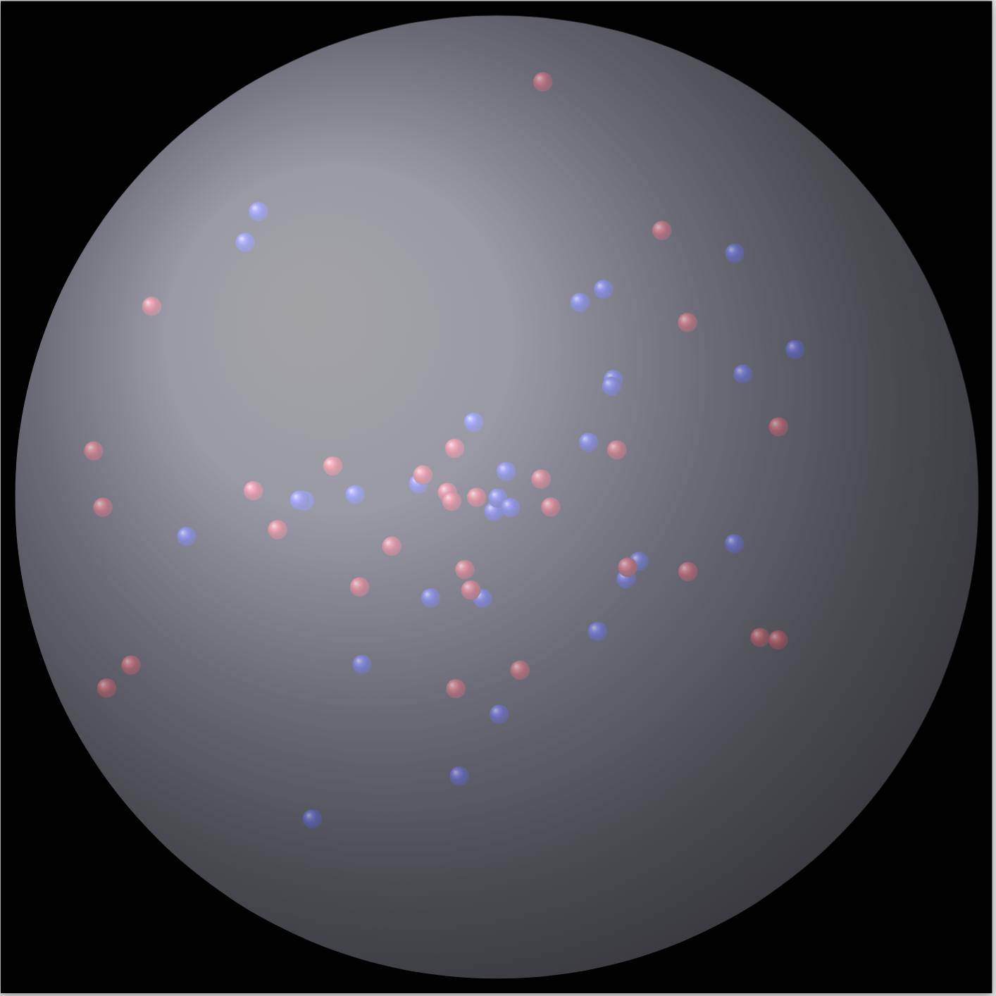
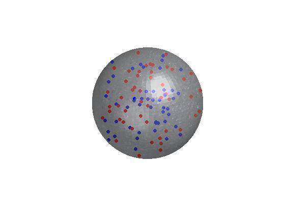
une autre solution avec Matlab.
[x,y,z] = sphere(50);
[img] = imread('crystal.jpg');

figure('Color',[0 0 0]);
surf(x,y,z,img,'edgeColor','none','FaceAlpha',.6,'FaceColor','texturemap')
hold on;

i = 0;
while i<100
    px = randn();
    py = randn();
    pz = randn();
    d = pdist([0 0 0; px py pz],'euclidean');
    if d<1
        if mod(i,2)==0
            scatter3(px, py, pz,30,'ro','filled');
        else
            scatter3(px, py, pz,30,'bo','filled');
        end
        i = i+1;
    end
end

hold off;
camlight;

axis equal;
axis off;
sortie:
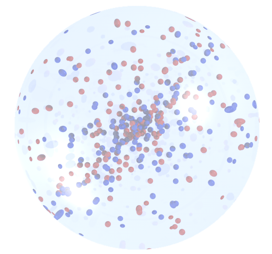
en Javascript avec d3.js: http://jsfiddle.net/jjcosare/rggn86aj/6 / ou > exécuter L'extrait de Code
utile pour la publication en ligne.
var particleChangePerMs = 1000;
var particleTotal = 250;
var particleSizeInRelationToCircle = 75;

var svgWidth = (window.innerWidth > window.innerHeight) ? window.innerHeight : window.innerWidth;
var svgHeight = (window.innerHeight > window.innerWidth) ? window.innerWidth : window.innerHeight;

var circleX = svgWidth / 2;
var circleY = svgHeight / 2;
var circleRadius = (circleX / 4) + (circleY / 4);
var circleDiameter = circleRadius * 2;

var particleX = function() {
  return Math.floor(Math.random() * circleDiameter) + circleX - circleRadius;
};
var particleY = function() {
  return Math.floor(Math.random() * circleDiameter) + circleY - circleRadius;
};
var particleRadius = function() {
  return circleDiameter / particleSizeInRelationToCircle;
};
var particleColorList = [
  'blue',
  'red'
];
var particleColor = function() {
  return "url(#" + particleColorList[Math.floor(Math.random() * particleColorList.length)] + "Gradient)";
};

var svg = d3.select("#quantumBall")
  .append("svg")
  .attr("width", svgWidth)
  .attr("height", svgHeight);

var blackGradient = svg.append("svg:defs")
  .append("svg:radialGradient")
  .attr("id", "blackGradient")
  .attr("cx", "50%")
  .attr("cy", "50%")
  .attr("radius", "90%")

blackGradient.append("svg:stop")
  .attr("offset", "80%")
  .attr("stop-color", "black")

blackGradient.append("svg:stop")
  .attr("offset", "100%")
  .attr("stop-color", "grey")

var redGradient = svg.append("svg:defs")
  .append("svg:linearGradient")
  .attr("id", "redGradient")
  .attr("x1", "0%")
  .attr("y1", "0%")
  .attr("x2", "100%")
  .attr("y2", "100%")
  .attr("spreadMethod", "pad");

redGradient.append("svg:stop")
  .attr("offset", "0%")
  .attr("stop-color", "red")
  .attr("stop-opacity", 1);

redGradient.append("svg:stop")
  .attr("offset", "100%")
  .attr("stop-color", "pink")
  .attr("stop-opacity", 1);

var blueGradient = svg.append("svg:defs")
  .append("svg:linearGradient")
  .attr("id", "blueGradient")
  .attr("x1", "0%")
  .attr("y1", "0%")
  .attr("x2", "100%")
  .attr("y2", "100%")
  .attr("spreadMethod", "pad");

blueGradient.append("svg:stop")
  .attr("offset", "0%")
  .attr("stop-color", "blue")
  .attr("stop-opacity", 1);

blueGradient.append("svg:stop")
  .attr("offset", "100%")
  .attr("stop-color", "skyblue")
  .attr("stop-opacity", 1);

svg.append("circle")
  .attr("r", circleRadius)
  .attr("cx", circleX)
  .attr("cy", circleY)
  .attr("fill", "url(#blackGradient)");

function isParticleInQuantumBall(particle) {
  var x1 = circleX;
  var y1 = circleY;
  var r1 = circleRadius;
  var x0 = particle.x;
  var y0 = particle.y;
  var r0 = particle.radius;
  return Math.sqrt((x1 - x0) * (x1 - x0) + (y1 - y0) * (y1 - y0)) < (r1 - r0);
};

function randomizedParticles() {
  d3.selectAll("svg > .particle").remove();
  var particle = {};
  particle.radius = particleRadius();
  for (var i = 0; i < particleTotal;) {
    particle.x = particleX();
    particle.y = particleY();
    particle.color = particleColor();
    if (isParticleInQuantumBall(particle)) {
      svg.append("circle")
        .attr("class", "particle")
        .attr("cx", particle.x)
        .attr("cy", particle.y)
        .attr("r", particle.radius)
        .attr("fill", particle.color);
      i++;
    }
  }
}

setInterval(randomizedParticles, particleChangePerMs);
<script src="https://cdnjs.cloudflare.com/ajax/libs/d3/3.4.11/d3.min.js"></script>
<div id="quantumBall"></div> dans R Vous pouvez utiliser la fonction rasterImage pour ajouter à un tracé actuel, vous pouvez soit créer/télécharger une belle image d'une boule de cristal et la charger dans R (voir png, EBImage, ou d'autres paquets) puis la rendre semi-transparente et utiliser rasterImage pour l'ajouter au tracé actuel. Je voudrais probablement tracer vos 2 points colorés d'abord, puis faire l'image de la balle au-dessus du dessus (avec transparence ils seront encore visibles et ressemblent à ils sont à l'intérieur).
un plus simple l'approche (bien que probablement pas aussi beau) est de juste dessiner un cercle gris semi-transparent en utilisant la fonction polygon pour représenter la balle.
si vous voulez le faire en 3 dimensions, regardez le paquet rgl, voici un exemple de base:
library(rgl)
open3d()
spheres3d(0,0,0, radius=1, color='lightgrey', alpha=0.2)
spheres3d(c(.3,-.3),c(-.2,.4),c(.1,.2), color=c('red','blue'),
     alpha=1, radius=0.15)