Comment puis-je spécifier un linestyle de type flèche dans Matplotlib?
je voudrais afficher un ensemble de xy-données dans Matplotlib de manière à indiquer un chemin particulier. Idéalement, le linestyle serait modifié pour utiliser un patch de type flèche. J'ai créé une maquette, illustrée ci-dessous (en utilisant Omnigraphsketcher). Il semble que je devrais être en mesure d'outrepasser l'un des communs linestyle déclarations ('-','--', ':', etc) à cet effet.
notez que je ne veux pas simplement connecter chaque point de données avec une flèche unique- - - les données réelles les points ne sont pas uniformément espacés et j'ai besoin d'un espacement constant entre les flèches.
4 réponses
Voici un point de départ:
marchez le long de votre ligne à pas fixes (
aspacedans mon exemple ci-dessous) .A. Il s'agit de prendre des mesures le long des segments de ligne créés par deux ensembles de points (
x1,y1) et (x2,y2).B. Si votre Pas est plus long que le segment de ligne, passez à la série suivante de points.
à ce point, déterminez l'angle de la ligne.
Dessiner une flèche avec une inclinaison correspondant à l'angle.
j'ai écrit un petit script pour montrer ceci:
import numpy as np
import matplotlib.pyplot as plt

fig = plt.figure()
axes = fig.add_subplot(111)

# my random data
scale = 10
np.random.seed(101)
x = np.random.random(10)*scale
y = np.random.random(10)*scale

# spacing of arrows
aspace = .1 # good value for scale of 1
aspace *= scale

# r is the distance spanned between pairs of points
r = [0]
for i in range(1,len(x)):
    dx = x[i]-x[i-1]
    dy = y[i]-y[i-1]
    r.append(np.sqrt(dx*dx+dy*dy))
r = np.array(r)

# rtot is a cumulative sum of r, it's used to save time
rtot = []
for i in range(len(r)):
    rtot.append(r[0:i].sum())
rtot.append(r.sum())

arrowData = [] # will hold tuples of x,y,theta for each arrow
arrowPos = 0 # current point on walk along data
rcount = 1
while arrowPos < r.sum():
    x1,x2 = x[rcount-1],x[rcount]
    y1,y2 = y[rcount-1],y[rcount]
    da = arrowPos-rtot[rcount]
    theta = np.arctan2((x2-x1),(y2-y1))
    ax = np.sin(theta)*da+x1
    ay = np.cos(theta)*da+y1
    arrowData.append((ax,ay,theta))
    arrowPos+=aspace
    while arrowPos > rtot[rcount+1]:
        rcount+=1
        if arrowPos > rtot[-1]:
            break

# could be done in above block if you want
for ax,ay,theta in arrowData:
    # use aspace as a guide for size and length of things
    # scaling factors were chosen by experimenting a bit
    axes.arrow(ax,ay,
               np.sin(theta)*aspace/10,np.cos(theta)*aspace/10,
               head_width=aspace/8)


axes.plot(x,y)
axes.set_xlim(x.min()*.9,x.max()*1.1)
axes.set_ylim(y.min()*.9,y.max()*1.1)

plt.show()
cet exemple donne cette figure:
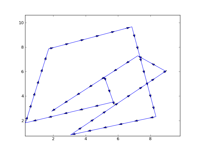
Il y a beaucoup de place à l'amélioration, pour commencer:
- On peut utiliser FancyArrowPatch pour personnaliser l'apparence des flèches.
- on peut ajouter un test supplémentaire quand créer les flèches pour s'assurer qu'elles ne s'étendent pas au-delà de la ligne. Cela s'applique aux flèches créées au sommet ou près d'un sommet où la ligne change brusquement de direction. C'est le cas pour la plupart des points ci-dessus.
- on peut faire une méthode à partir de ce script qui fonctionnera dans un plus grand nombre de cas, c'est-à-dire la rendre plus portable.
en regardant cela, j'ai découvert le carquois méthode de traçage. Il pourrait être en mesure de remplacer le ci-dessus travail, mais il n'était pas immédiatement évident que cela était garanti.
Très belle réponse par Yann, mais en utilisant la flèche les flèches résultantes peuvent être affectées par le rapport d'aspect des axes et les limites. J'ai fait une version qui utilise des haches.annotate() à la place d'axes.flèche.)( Je l'inclus ici pour les autres à utiliser.
en bref ceci est utilisé pour tracer des flèches le long de vos lignes dans matplotlib. Le code est indiqué ci-dessous. Il peut encore être amélioré en ajoutant la possibilité d'avoir différentes pointes de flèche. Ici, j'ai seulement inclus le contrôle pour le largeur et longueur de la pointe de flèche.
import numpy as np
import matplotlib.pyplot as plt


def arrowplot(axes, x, y, narrs=30, dspace=0.5, direc='pos', \
                          hl=0.3, hw=6, c='black'):
    ''' narrs  :  Number of arrows that will be drawn along the curve

        dspace :  Shift the position of the arrows along the curve.
                  Should be between 0. and 1.

        direc  :  can be 'pos' or 'neg' to select direction of the arrows

        hl     :  length of the arrow head

        hw     :  width of the arrow head

        c      :  color of the edge and face of the arrow head
    '''

    # r is the distance spanned between pairs of points
    r = [0]
    for i in range(1,len(x)):
        dx = x[i]-x[i-1]
        dy = y[i]-y[i-1]
        r.append(np.sqrt(dx*dx+dy*dy))
    r = np.array(r)

    # rtot is a cumulative sum of r, it's used to save time
    rtot = []
    for i in range(len(r)):
        rtot.append(r[0:i].sum())
    rtot.append(r.sum())

    # based on narrs set the arrow spacing
    aspace = r.sum() / narrs

    if direc is 'neg':
        dspace = -1.*abs(dspace)
    else:
        dspace = abs(dspace)

    arrowData = [] # will hold tuples of x,y,theta for each arrow
    arrowPos = aspace*(dspace) # current point on walk along data
                                 # could set arrowPos to 0 if you want
                                 # an arrow at the beginning of the curve

    ndrawn = 0
    rcount = 1
    while arrowPos < r.sum() and ndrawn < narrs:
        x1,x2 = x[rcount-1],x[rcount]
        y1,y2 = y[rcount-1],y[rcount]
        da = arrowPos-rtot[rcount]
        theta = np.arctan2((x2-x1),(y2-y1))
        ax = np.sin(theta)*da+x1
        ay = np.cos(theta)*da+y1
        arrowData.append((ax,ay,theta))
        ndrawn += 1
        arrowPos+=aspace
        while arrowPos > rtot[rcount+1]:
            rcount+=1
            if arrowPos > rtot[-1]:
                break

    # could be done in above block if you want
    for ax,ay,theta in arrowData:
        # use aspace as a guide for size and length of things
        # scaling factors were chosen by experimenting a bit

        dx0 = np.sin(theta)*hl/2. + ax
        dy0 = np.cos(theta)*hl/2. + ay
        dx1 = -1.*np.sin(theta)*hl/2. + ax
        dy1 = -1.*np.cos(theta)*hl/2. + ay

        if direc is 'neg' :
          ax0 = dx0
          ay0 = dy0
          ax1 = dx1
          ay1 = dy1
        else:
          ax0 = dx1
          ay0 = dy1
          ax1 = dx0
          ay1 = dy0

        axes.annotate('', xy=(ax0, ay0), xycoords='data',
                xytext=(ax1, ay1), textcoords='data',
                arrowprops=dict( headwidth=hw, frac=1., ec=c, fc=c))


    axes.plot(x,y, color = c)
    axes.set_xlim(x.min()*.9,x.max()*1.1)
    axes.set_ylim(y.min()*.9,y.max()*1.1)


if __name__ == '__main__':
    fig = plt.figure()
    axes = fig.add_subplot(111)

    # my random data
    scale = 10
    np.random.seed(101)
    x = np.random.random(10)*scale
    y = np.random.random(10)*scale
    arrowplot(axes, x, y )

    plt.show()
Le résultat peut être vu ici:
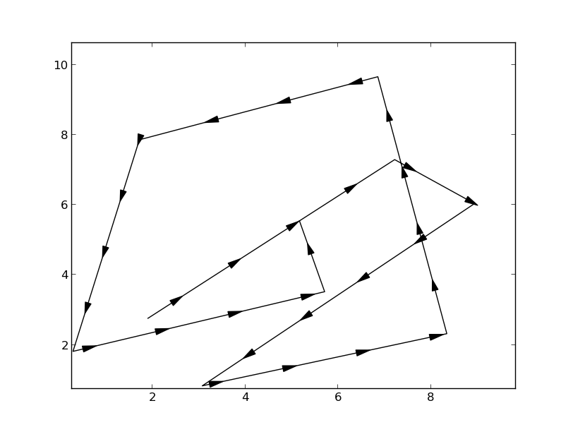
version vectorisée de la réponse de Yann:
import numpy as np
import matplotlib.pyplot as plt

def distance(data):
    return np.sum((data[1:] - data[:-1]) ** 2, axis=1) ** .5

def draw_path(path):
    HEAD_WIDTH = 2
    HEAD_LEN = 3

    fig = plt.figure()
    axes = fig.add_subplot(111)

    x = path[:,0]
    y = path[:,1]
    axes.plot(x, y)

    theta = np.arctan2(y[1:] - y[:-1], x[1:] - x[:-1])
    dist = distance(path) - HEAD_LEN

    x = x[:-1]
    y = y[:-1]
    ax = x + dist * np.sin(theta)
    ay = y + dist * np.cos(theta)

    for x1, y1, x2, y2 in zip(x,y,ax-x,ay-y):
        axes.arrow(x1, y1, x2, y2, head_width=HEAD_WIDTH, head_length=HEAD_LEN)
    plt.show()
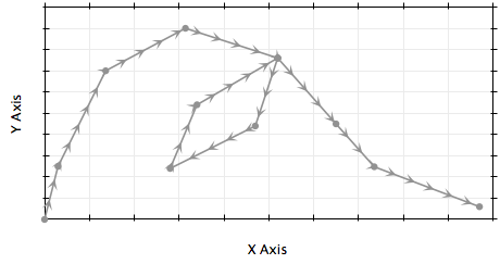
Voici une version modifiée et simplifiée du code de Duarte. J'ai eu des problèmes quand j'ai lancé son code avec différents ensembles de données et rapports d'aspect, donc je l'ai nettoyé et utilisé FancyArrowPatches pour les flèches. Remarque l'exemple de la parcelle a une échelle de 1 000 000 de fois différent de x que de y.
j'ai aussi changé pour dessiner la flèche dans affichage coordonnées de façon à ce que les différences d'échelle sur les axes x et y ne changent pas la longueur des flèches.
en cours de route j'ai trouvé un bug dans le FancyArrowPatch de matplotlib qui explose en traçant une flèche purement verticale. J'ai trouvé une solution qui est dans mon code.
import numpy as np
import matplotlib.pyplot as plt
import matplotlib.patches as patches


def arrowplot(axes, x, y, nArrs=30, mutateSize=10, color='gray', markerStyle='o'):
    '''arrowplot : plots arrows along a path on a set of axes
        axes   :  the axes the path will be plotted on
        x      :  list of x coordinates of points defining path
        y      :  list of y coordinates of points defining path
        nArrs  :  Number of arrows that will be drawn along the path
        mutateSize :  Size parameter for arrows
        color  :  color of the edge and face of the arrow head
        markerStyle : Symbol

        Bugs: If a path is straight vertical, the matplotlab FanceArrowPatch bombs out.
          My kludge is to test for a vertical path, and perturb the second x value
          by 0.1 pixel. The original x & y arrays are not changed

        MHuster 2016, based on code by
    '''
    # recast the data into numpy arrays
    x = np.array(x, dtype='f')
    y = np.array(y, dtype='f')
    nPts = len(x)

    # Plot the points first to set up the display coordinates
    axes.plot(x,y, markerStyle, ms=5, color=color)

    # get inverse coord transform
    inv = ax.transData.inverted()

    # transform x & y into display coordinates
    # Variable with a 'D' at the end are in display coordinates
    xyDisp = np.array(axes.transData.transform(zip(x,y)))
    xD = xyDisp[:,0]
    yD = xyDisp[:,1]

    # drD is the distance spanned between pairs of points
    # in display coordinates
    dxD = xD[1:] - xD[:-1]
    dyD = yD[1:] - yD[:-1]
    drD = np.sqrt(dxD**2 + dyD**2)

    # Compensating for matplotlib bug
    dxD[np.where(dxD==0.0)] = 0.1


    # rtotS is the total path length
    rtotD = np.sum(drD)

    # based on nArrs, set the nominal arrow spacing
    arrSpaceD = rtotD / nArrs

    # Loop over the path segments
    iSeg = 0
    while iSeg < nPts - 1:
        # Figure out how many arrows in this segment.
        # Plot at least one.
        nArrSeg = max(1, int(drD[iSeg] / arrSpaceD + 0.5))
        xArr = (dxD[iSeg]) / nArrSeg # x size of each arrow
        segSlope = dyD[iSeg] / dxD[iSeg]
        # Get display coordinates of first arrow in segment
        xBeg = xD[iSeg]
        xEnd = xBeg + xArr
        yBeg = yD[iSeg]
        yEnd = yBeg + segSlope * xArr
        # Now loop over the arrows in this segment
        for iArr in range(nArrSeg):
            # Transform the oints back to data coordinates
            xyData = inv.transform(((xBeg, yBeg),(xEnd,yEnd)))
            # Use a patch to draw the arrow
            # I draw the arrows with an alpha of 0.5
            p = patches.FancyArrowPatch(
                xyData[0], xyData[1],
                arrowstyle='simple',
                mutation_scale=mutateSize,
                color=color, alpha=0.5)
            axes.add_patch(p)
            # Increment to the next arrow
            xBeg = xEnd
            xEnd += xArr
            yBeg = yEnd
            yEnd += segSlope * xArr
        # Increment segment number
        iSeg += 1

if __name__ == '__main__':
    import numpy as np
    import matplotlib.pyplot as plt
    fig = plt.figure()
    ax = fig.add_subplot(111)
    # my random data
    xScale = 1e6
    np.random.seed(1)
    x = np.random.random(10) * xScale
    y = np.random.random(10)
    arrowplot(ax, x, y, nArrs=4*(len(x)-1), mutateSize=10, color='red')
    xRng = max(x) - min(x)
    ax.set_xlim(min(x) - 0.05*xRng, max(x) + 0.05*xRng)
    yRng = max(y) - min(y)
    ax.set_ylim(min(y) - 0.05*yRng, max(y) + 0.05*yRng)
    plt.show()
